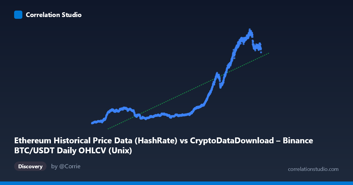
Ethereum Historical Price Data (HashRate) vs CryptoDataDownload – Binance BTC/USDT Daily OHLCV (Unix)
- Pearson correlation (r)
- 0.83
- Spearman correlation
- 0.7965
- p-value
- 0
- Sample size (n)
- 1855
- 95% confidence interval
- 0.8153 to 0.8437
- Granger causality
- X → Y
- Granger optimal lag
- 2
AI analysis
Analysis: Time-Based Relationship Between Two Variables
Important caveat first: Despite the axis labels referencing "Ethereum" and "BTC/USDT HashRate/OHLCV," the X-axis is actually a raw Unix timestamp (values in the 1.5–1.66 trillion range, corresponding to dates from late 2017 to September 2022). This is fundamentally a time series analysis of Y against time, not a comparison between two independent economic variables. This context should reframe the entire interpretation below.
1. What the Visualization Reveals
The scatterplot shows Y (ranging from ~83 to ~1,065, likely a price or valuation metric) plotted against time. The sample points reveal a clear long-term upward trajectory: values hover in the 100–250 range through 2018–2021, then climb sharply through 2021–2022, reaching 900–1,065 by mid-2022. This is not a linear relationship in the traditional sense but rather a growth trend with distinct phases — a relatively flat/low-volatility period followed by a steep ascent.
2. Strength, Direction, and Statistical Confidence
The correlation coefficient (r = 0.83) indicates a strong positive relationship, with r² = 0.689 meaning 69% of the variance in Y is explained by time, leaving 31% attributable to other factors (volatility, cyclical dynamics, external shocks). The 95% CI [0.815, 0.844] is tight given the large sample (n=1,855), and p≈0 confirms this relationship is statistically robust, not due to chance. However, the Granger causality result is the most nuanced piece: X "causes" Y at only marginal significance (F=3.19, p=0.041) — weak evidence at best — while Y does not predict X (p=0.31). Since X is literally time, this "causality" result is somewhat tautological (time trivially "precedes" Y) and should not be over-interpreted as a meaningful predictive mechanism.
3. Notable Patterns and Outliers
The data shows clear regime clustering rather than uniform linear growth: - 2017–2021 "low regime": Y values cluster tightly between 100–250, suggesting a period of relative stability or slow growth. - 2021–2022 "high regime": A steep breakout occurs, with Y values jumping to 400–1,065, indicating a possible bull-market or bubble-like phase. - The transition appears abrupt rather than gradual, suggesting a structural break or regime shift rather than smooth linear growth — this is typical of crypto asset price behavior and should raise flags about using a single linear model across the whole period.
4. Confounding Factors and Caveats
Several critical caveats apply: - Spurious/mechanical correlation risk: Since X is time itself, r² here reflects a trend-fitting exercise, not a causal economic relationship between two independent variables. Any monotonically trending series will show artificially high correlation with time. - Non-stationarity: Both series (time and Y) exhibit trends, which inflates correlation and can produce misleading Granger causality results — a well-known issue in financial time series (spurious regression problem, per Granger & Newbo). - Metadata confusion: The column labels are inconsistent/mismatched (Ethereum vs. BTC/USDT, HashRate vs. OHLCV), suggesting possible data pipeline errors that should be resolved before drawing substantive conclusions. - Volatility clustering: Crypto prices exhibit heteroskedasticity — variance is not constant across time, violating linear regression assumptions.
5. Actionable Recommendations
1. Clarify data provenance — resolve the mismatched column/dataset labels before treating this as a meaningful bivariate analysis. 2. Detrend and test for stationarity (e.g., ADF test) before relying on correlation/Granger results; consider differencing or log-transforming Y given its exponential-looking growth. 3. Segment the analysis by regime (pre-2021 vs. 2021–2022) to check if the relationship holds within each phase or is purely driven by the late breakout. 4. Replace linear regression with a model suited to exponential/logistic growth patterns, given the visible inflection point. 5. If the actual intent was to compare two distinct market variables (e.g., BTC price vs. ETH hashrate), re-pull correctly labeled data and rerun the analysis, since the current setup essentially measures "Y vs. time," not "Y vs. X variable of interest."
X dataset: CryptoDataDownload – Binance BTC/USDT Daily OHLCV
Y dataset: Ethereum Historical Price Data
Part of experiment: Bitcoin - CryptoDataDownload – Binance BTC/USDT Daily OHLCV vs Ethereum Historical Price Data