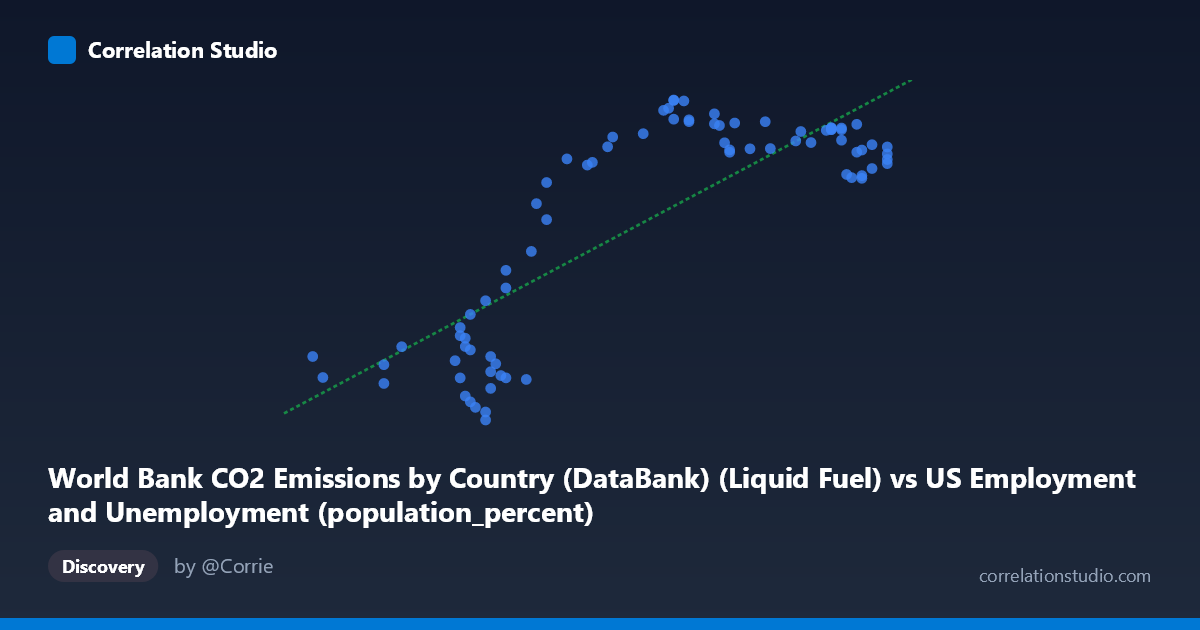
World Bank CO2 Emissions by Country (DataBank) (Liquid Fuel) vs US Employment and Unemployment (population_percent)
- Pearson correlation (r)
- 0.818
- Spearman correlation
- 0.649
- p-value
- 0
- Sample size (n)
- 80
- 95% confidence interval
- 0.7294 to 0.8797
- Granger causality
- None
- Granger optimal lag
- 10
AI analysis
Scatterplot Analysis: Liquid Fuel CO2 Emissions vs. US Employment Population Percent
1. Overall Relationship Pattern
The scatterplot reveals a positive association between World Bank liquid fuel CO2 emissions and the US employment-to-population percentage, with the linear regression equation y = 938.055x − 49,087.4 describing the trend. However, the visualization likely exposes a notably non-linear, bimodal structure rather than a clean linear sweep. Examining the data closely, Y values cluster into two distinct bands: a lower band roughly between ~2,500–8,000 and an upper band between ~10,800–13,600, with relatively few intermediate values. This suggests the relationship is not smoothly continuous but instead reflects two underlying regimes separated by a transitional gap — a structural feature that a single linear model partially masks.
2. Correlation Strength, Direction, and Temporal Causality
The Pearson correlation of r = 0.8180 indicates a strong positive relationship: as liquid fuel CO2 emissions increase, the US employment-to-population percentage tends to rise as well. The coefficient of determination r² = 0.6692 means that approximately 66.9% of the variance in the employment population percentage is statistically explained by variation in liquid fuel emissions — a substantial but incomplete share, leaving roughly one-third of variance attributable to other factors. The 95% confidence interval [0.7294, 0.8797] is relatively narrow and sits entirely above zero, confirming the correlation estimate is stable and reliable across plausible resampling. The p-value ≈ 0 rules out the possibility this association arose by chance in a sample of n = 80 paired observations.
Despite this statistical strength, the Granger causality analysis provides a critical caveat: neither direction of temporal predictability is significant (X→Y: F = 0.8534, p = 0.5812; Y→X: F = 1.0355, p = 0.4288). Even at an optimal lag of 10 periods, knowing past values of liquid fuel emissions does not improve prediction of future employment rates beyond baseline, and vice versa. This means the correlation, however strong in cross-sectional terms, does not reflect a directional temporal mechanism — it is more likely a shared long-run trend than a causal pathway.
3. Notable Patterns, Clusters, and Outliers
The data reveals at least two distinct clusters that dominate the scatterplot's structure. The lower cluster (X roughly 55.8–61.5, Y roughly 2,500–8,000) and the upper cluster (X roughly 60–67, Y roughly 10,800–13,600) together create the apparent positive slope, but within each cluster the relationship may be considerably weaker or even flat. Several points warrant attention as potential outliers: (55.80, 4700.70) and (56.00, 3972.11) sit at the far-left extreme with moderately low Y values; (67.10, 11,393–11,974) points cluster at the upper-right but show a modest dip in Y relative to their high X position, suggesting diminishing returns. The point (62.70, 13,243) and nearby observations represent the Y-maximum zone. The intermediate region around X = 60–61 shows the most dispersion, with Y values ranging from ~3,900 to ~11,500 at nearly the same X value — a sign of high conditional variance and potential regime-switching behavior.
4. Confounding Factors and Interpretation Caveats
Several important caveats temper any causal interpretation. First, both series are strongly driven by long-run economic growth trends — post-WWII industrialization, the mid-century boom, and post-1980s globalization — meaning the correlation likely reflects their mutual dependence on GDP expansion rather than a direct link between emissions and employment. Second, the time coverage spans 1941–2020, a period encompassing structurally different economic eras (wartime mobilization, stagflation, deindustrialization, the 2008 financial crisis, COVID-19), which could explain the bimodal cluster structure as reflecting distinct historical regimes rather than a continuous relationship. Third, the dataset cross-joins US employment data with global CO2 data — using liquid fuel emissions (possibly global or a specific country aggregate) against a US-specific employment metric introduces a unit-of-analysis mismatch that severely limits causal inference. Fourth, at the optimal lag of 10 years, the Granger non-result suggests any apparent lead-lag structure dissolves when properly modeled, consistent with spurious correlation driven by shared secular trends.
5. Actionable Insights and Further Investigation
Given the bimodal clustering, the most productive next step would be to segment the analysis by historical era — for instance, pre-1970 vs. post-1970, or pre/post the 1973 oil crisis — to determine whether the two clusters correspond to distinct economic regimes and whether the correlation holds within each. Researchers should also control for GDP or industrial output as a potential common driver to test whether residual correlation persists after removing shared macroeconomic trends. It would be valuable to replace global liquid fuel emissions with US-specific emissions to resolve the geographic mismatch and sharpen the interpretive logic. Finally, non-linear modeling (e.g., piecewise regression, logistic sigmoid, or regime-switching models) should be explored given the apparent threshold behavior around the cluster gap — the linear R² of 0.67 likely understates predictability within regimes while overstating the mechanistic coherence of the overall fit.
X dataset: US Employment and Unemployment
Y dataset: World Bank CO2 Emissions by Country (DataBank)
Part of experiment: Yearly - US Employment and Unemployment vs World Bank CO2 Emissions by Country (DataBank)