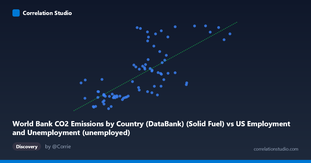
World Bank CO2 Emissions by Country (DataBank) (Solid Fuel) vs US Employment and Unemployment (unemployed)
- Pearson correlation (r)
- 0.7218
- Spearman correlation
- 0.7338
- p-value
- 0
- Sample size (n)
- 80
- 95% confidence interval
- 0.5967 to 0.8126
- Granger causality
- None
- Granger optimal lag
- 10
AI analysis
Scatterplot Analysis: Solid Fuel CO2 Emissions vs. US Unemployment
1. Overall Relationship Pattern
The scatterplot reveals a moderately positive relationship between World Bank solid fuel CO2 emissions and US unemployment figures across the 1941–2020 timeframe. The linear regression (y = 1.490x + 9040.01) captures a general upward trend, but the scatter around this line is notably wide, suggesting the relationship is far from deterministic. Visually, the data points form a loose cloud with some clustering in the lower-left quadrant (lower emissions, lower unemployment) and a spread of points extending toward higher values on both axes, consistent with a correlation that is real but noisy.
2. Correlation Strength, Direction, and Causality
The Pearson correlation of r = 0.72 indicates a moderate-to-strong positive association, but the R² of 0.521 is the more sobering statistic — only about 52% of the variance in unemployment is explained by solid fuel CO2 emissions, meaning nearly half the variation remains unexplained by this single predictor. The 95% confidence interval of [0.597, 0.813] is reasonably tight and does not include zero, and the p-value of 4.24×10⁻¹⁴ confirms the correlation is highly statistically significant, making it very unlikely to be a chance artifact given n = 80 paired observations. However, the Granger causality tests are unambiguous in their null result: neither X→Y (F = 0.916, p = 0.526) nor Y→X (F = 0.982, p = 0.471) reaches significance even at an optimal lag of 10 periods. This means that knowing past values of CO2 emissions does not improve forecasts of unemployment beyond what unemployment's own history provides, and vice versa — the correlation is associative, not temporally predictive.
3. Notable Patterns, Clusters, and Outliers
Several structural features are visible in the data. A dense cluster exists around X ≈ 2,000–5,000 and Y ≈ 10,000–14,000, likely corresponding to the mid-20th century period of lower industrial activity and lower unemployment baselines. A second, more dispersed cluster emerges at X ≈ 6,000–9,000 and Y ≈ 15,000–30,000, reflecting later decades of both higher emissions and higher absolute unemployment counts. Several prominent outliers deserve attention: the point at (670, 16,274) shows relatively high unemployment despite very low CO2 emissions, potentially reflecting an early wartime anomaly; conversely, points near (6,001, 30,698) and (6,314, 30,479) show extreme unemployment values at moderate emissions levels, possibly capturing recession-era peaks (e.g., early 1980s or 2008–2009). The point at (14,825, 29,066) represents the high-emissions extreme and sits below the regression line, suggesting diminishing returns at the upper end. The relationship also appears to show mild non-linearity or heteroscedasticity — variance in Y appears to increase at higher X values, which a simple linear model may underfit.
4. Confounding Factors and Interpretive Caveats
This correlation almost certainly reflects a shared common driver: long-run population and economic growth. As the US (and global) economy expanded over the 20th century, both industrial energy consumption (driving solid fuel CO2 emissions) and the absolute number of unemployed persons grew simply because the labor force and industrial base grew. This is a classic spurious correlation driven by secular trends — two upward-trending time series will often correlate strongly without any causal mechanism. The fact that the dataset conflates two different source databases (US BLS employment data and World Bank global CO2 data) introduces additional noise from definitional and methodological inconsistencies. The 80-year time span also spans fundamentally different economic regimes (wartime mobilization, postwar expansion, stagflation, deindustrialization, financialization), making stationarity assumptions questionable. The Granger causality null result further reinforces that this should not be interpreted as a mechanistic relationship.
5. Actionable Insights and Further Investigation
Given the moderate correlation without causal directionality, several follow-up analyses are warranted. First, detrending both series (e.g., using first differences or HP filtering) before computing correlation would test whether the relationship survives removal of shared growth trends — this is the most critical next step. Second, controlling for labor force size by using unemployment rate rather than absolute counts would normalize for population growth and likely weaken the correlation substantially. Third, examining sector-specific emissions (e.g., manufacturing vs. transportation) alongside industry-specific employment could reveal more mechanistically meaningful sub-relationships. Fourth, a structural break analysis (e.g., Chow test) around major economic disruptions (1973 oil shock, 2008 financial crisis, COVID-19) would clarify whether the relationship is stable or epoch-dependent. Finally, incorporating additional covariates such as GDP, energy prices, and trade openness in a multivariate framework would better isolate any genuine partial correlation between emissions and employment dynamics.
X dataset: US Employment and Unemployment
Y dataset: World Bank CO2 Emissions by Country (DataBank)
Part of experiment: Yearly - US Employment and Unemployment vs World Bank CO2 Emissions by Country (DataBank)