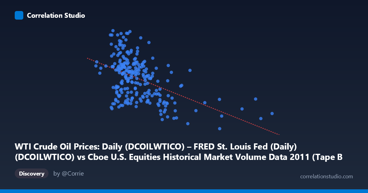
WTI Crude Oil Prices: Daily (DCOILWTICO) – FRED St. Louis Fed (Daily) (DCOILWTICO) vs Cboe U.S. Equities Historical Market Volume Data 2011 (Tape B Trade Count)
- Pearson correlation (r)
- -0.4891
- Spearman correlation
- -0.4243
- p-value
- 0
- Sample size (n)
- 252
- 95% confidence interval
- -0.5777 to -0.389
- Granger causality
- None
- Granger optimal lag
- 1
AI analysis
Analysis: WTI Crude Oil Prices vs. Cboe Tape B Trade Count (2011)
Relationship Overview The scatterplot reveals a moderate negative relationship between WTI crude oil prices (X-axis) and Cboe Tape B trade counts (Y-axis) across 252 trading days in 2011. As oil prices increase, equity trade counts on Tape B venues tend to decline, and vice versa. The linear regression equation (y = -3.77E-05x + 105.496) quantifies this inverse slope, meaning that for every $1,000 increase in the oil price index value, Tape B trade counts decrease by approximately 0.038 units. The relationship is visually discernible but noisy, with considerable scatter around the regression line, suggesting that oil prices are far from the sole driver of exchange trade volume.
Correlation Strength and Statistical Significance The Pearson correlation of r = -0.489 indicates a moderate negative association. However, the r² value of 0.239 tells a more sobering story: oil prices explain only ~24% of the variance in Tape B trade counts, leaving roughly 76% of variation unexplained by this single variable. The 95% confidence interval for r of [-0.578, -0.389] is meaningfully negative throughout, confirming that the direction of the relationship is reliable, and the p-value of 2.22E-16 confirms the result is highly statistically significant given the large population (N = 3,780). That said, statistical significance here is substantially driven by the large sample size and should not be conflated with practical or economic significance. Critically, the Granger causality tests show no significant predictive directionality: neither X→Y (F = 0.005, p = 0.945) nor Y→X (F = 3.14, p = 0.078) clears the conventional 0.05 threshold at lag-1, meaning that past oil prices do not statistically predict future trade counts, nor vice versa. This absence of temporal predictive power is an important caveat — the correlation is contemporaneous and associative, not directionally causal.
Notable Patterns and Outliers Several features stand out in the data. The bulk of observations cluster in the $150,000–$400,000 oil price range with trade counts between ~85–108, forming the core of the negative trend. There are visible outliers at higher oil price values (e.g., points near $495,000–$832,000) that appear to pull the regression but show somewhat scattered Y-values, potentially weakening the linear fit at the extremes. A point near (556,197, 85.48) and another at approximately (832,000) in the full dataset represent high-leverage observations worth examining. There is also a fan-like spread at lower X values, where trade counts show high variance (~85–113), suggesting that when oil prices are lower, other market-structure or volatility factors dominate trade count behavior. No strong non-linear curvature is evident, though the wide scatter hints that a linear model may be a simplification.
Confounding Factors and Interpretive Caveats Several important caveats apply. First, 2011 was a particularly volatile year for both oil markets (Arab Spring, Libya conflict) and equities (U.S. debt ceiling crisis, European sovereign debt fears), meaning market-wide stress periods likely drove both variables simultaneously — a classic common-cause confound. Elevated market uncertainty increases equity trading volume while simultaneously affecting oil prices, which could manufacture or inflate the observed correlation. Second, Tape B specifically covers regional exchanges (NYSE American, etc.), so volume shifts between Tape A, B, and C venues due to exchange competition or regulatory changes could introduce structural noise unrelated to oil. Third, the dataset spans only one calendar year, limiting generalizability. Finally, the axes appear to use raw numerical identifiers rather than standard units (e.g., $/barrel for oil), so the scale interpretation requires validation against the original FRED series.
Actionable Insights and Further Investigation Given that oil prices explain only ~24% of trade count variance and show no Granger-causal relationship, practitioners should avoid using oil prices as a standalone predictor of Tape B volume in trading models. However, the consistent negative association warrants further exploration. Recommended next steps include: (1) extending the analysis to multiple years to test whether the 2011 relationship persists or is regime-specific; (2) controlling for the CBOE VIX as a mediating variable, since volatility likely drives both oil price swings and equity trading intensity; (3) decomposing trade counts by market cap tier or sector to see whether energy-sector equities disproportionately drive the Tape B pattern; and (4) testing non-linear or regime-switching models (e.g., separating high-volatility from low-volatility periods) to assess whether the correlation strengthens under specific market conditions. The near-significant Y→X Granger result (p = 0.077) also merits re-testing at longer lags, as equity market activity may influence oil price discovery with a slightly delayed effect.
X dataset: Cboe U.S. Equities Historical Market Volume Data 2011
Y dataset: WTI Crude Oil Prices: Daily (DCOILWTICO) – FRED St. Louis Fed (Daily)
Part of experiment: Daily - Cboe U.S. Equities Historical Market Volume Data 2011 vs WTI Crude Oil Prices: Daily (DCOILWTICO) – FRED St. Louis Fed (Daily)