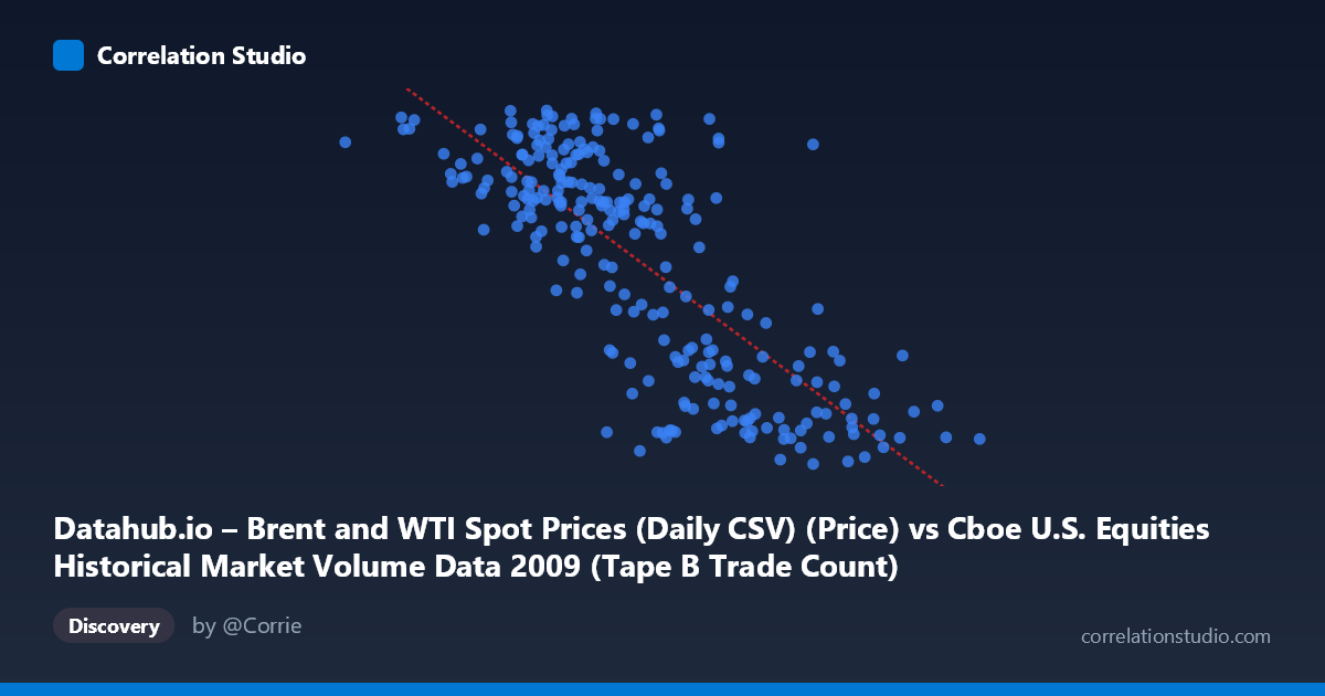
Datahub.io – Brent and WTI Spot Prices (Daily CSV) (Price) vs Cboe U.S. Equities Historical Market Volume Data 2009 (Tape B Trade Count)
- Pearson correlation (r)
- -0.7718
- Spearman correlation
- -0.7447
- p-value
- 0
- Sample size (n)
- 252
- 95% confidence interval
- -0.8175 to -0.7166
- Granger causality
- None
- Granger optimal lag
- 1
AI analysis
Analysis: Brent/WTI Oil Prices vs. Cboe Tape B Trade Count (2009)
Relationship Overview The scatterplot reveals a moderately strong negative relationship between daily U.S. equity market trade counts (Tape B) on the X-axis and Brent/WTI oil spot prices on the Y-axis across 2009. As trading volume activity increases, oil prices tend to be lower, and conversely, lower trade counts correspond with higher oil prices. The linear regression equation (y = -7.6372E-05x + 92.43) quantifies this inverse slope, suggesting that for every additional ~13,000 trades, oil prices decline by approximately $1/barrel. This pattern is visually apparent as a downward-sloping cloud of points spanning roughly $40–$78 per barrel against a wide trade count range.
Correlation Strength and Statistical Significance The Pearson correlation of r = -0.7718 indicates a strong negative association, and with r² = 0.5957, approximately 59.6% of the variance in oil prices is explained by trade count activity — a substantial explanatory share for financial time-series data. The 95% confidence interval of [-0.8175, -0.7166] is narrow and entirely negative, confirming the direction with high certainty. The p-value of effectively 0 (across N = 3,232) makes it statistically unambiguous that this correlation is not due to chance. However, the Granger causality results are striking in their absence: neither direction shows predictive power (X→Y: F = 0.0096, p = 0.922; Y→X: F = 1.956, p = 0.163). This critical finding means that while the two variables are strongly correlated contemporaneously, neither one temporally predicts the other at a one-period lag — the relationship is associative, not predictive in the causal-temporal sense.
Patterns, Clusters, and Outliers The data cloud shows a reasonably consistent linear trend but with notable heteroscedasticity — the spread of oil prices is wider at moderate trade counts (roughly 300,000–450,000) and tighter at the extremes. Several clusters are visible: a dense grouping around 300,000–400,000 trades with oil prices in the $60–$78 range (likely corresponding to the oil price recovery in the second half of 2009), and another cluster at 450,000–650,000 trades with prices compressed into the $40–$57 range (likely the depressed price environment of early 2009 post-financial crisis). A few notable outliers appear at the far right (e.g., 766,763 trades at $42.19 and 662,859 at $41.27) and at the lower-left extreme (81,703 trades at $75.15), which may reflect days of exceptional market stress or unusually thin trading sessions.
Confounding Factors and Caveats The 2009 timeframe is critical context: this was a year of extraordinary market recovery following the 2008 financial crisis. Both oil prices and equity trading volumes were heavily influenced by a single dominant macroeconomic narrative — risk appetite returning to markets. Higher fear/risk-off periods (early 2009) corresponded with cheap oil and paradoxically lower or higher volumes depending on the specific event. The apparent correlation may largely be a shared dependence on a third variable — macroeconomic sentiment or the VIX — rather than a direct relationship between trade counts and oil prices. Additionally, the axis labels appear potentially swapped from their dataset descriptions, warranting a data integrity check before drawing firm conclusions. Seasonality within 2009 and the structural break around March 2009 (market bottom) could be artificially inflating the correlation coefficient.
Actionable Insights and Further Investigation Given the strong correlation but absent Granger causality, analysts should not use trade count to forecast oil prices or vice versa in a trading strategy context. Instead, the relationship warrants investigation as a coincident indicator of broader market regime shifts. Recommended next steps include: (1) introducing a risk sentiment proxy (e.g., VIX, credit spreads) as a mediating variable to test whether the correlation disappears once market fear is controlled for; (2) segmenting the data by quarter to test whether the correlation is consistent throughout 2009 or driven by the Q1 recovery period; (3) testing non-linear models given the visual clustering, which may reveal threshold effects around key oil price levels ($50, $60/barrel); and (4) extending the dataset beyond 2009 to test whether this relationship persists in non-crisis years or was purely an artifact of the exceptional macroeconomic environment.
X dataset: Cboe U.S. Equities Historical Market Volume Data 2009
Y dataset: Datahub.io – Brent and WTI Spot Prices (Daily CSV)
Part of experiment: Daily - Cboe U.S. Equities Historical Market Volume Data 2009 vs Datahub.io – Brent and WTI Spot Prices (Daily CSV)