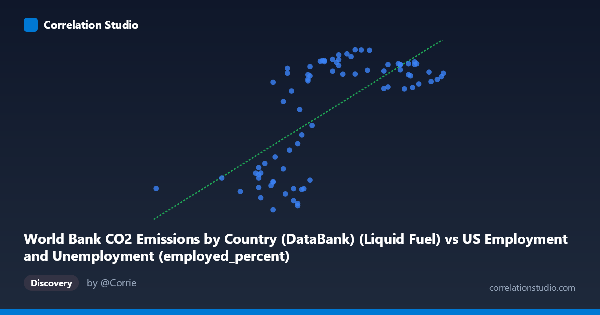
World Bank CO2 Emissions by Country (DataBank) (Liquid Fuel) vs US Employment and Unemployment (employed_percent)
- Pearson correlation (r)
- 0.6964
- Spearman correlation
- 0.6459
- p-value
- 0
- Sample size (n)
- 80
- 95% confidence interval
- 0.5628 to 0.7946
- Granger causality
- None
- Granger optimal lag
- 10
- Time coverage
- 1941-01-01 to 2020-01-01
AI analysis
Scatterplot Analysis: Liquid Fuel CO2 Emissions vs. US Employment Percentage
1. Overall Relationship Pattern
The scatterplot reveals a moderately positive relationship between World Bank liquid fuel CO2 emissions and US employment percentage, with a linear regression of y = 885.82x − 42,711.9. However, the data distribution is notably non-linear in character: rather than a smooth, continuous trend, the plot displays what appears to be a bimodal or sigmoidal clustering pattern, with a dense lower cluster of points (Y roughly 2,500–8,000) at lower X values and a second dense upper cluster (Y roughly 10,000–14,000) spanning a broader X range. This suggests the relationship may not be fundamentally linear, and the moderate r value may partly reflect transition between two distinct regimes rather than a uniform linear association.
2. Correlation Strength, Direction, and Causality
The Pearson correlation of r = 0.696 indicates a moderate-to-strong positive association, but the R² of 0.485 is the more sobering figure: only about 48.5% of the variance in employment percentage is explained by liquid fuel CO2 emissions, leaving over half the variance attributable to other factors. The 95% confidence interval for r [0.563, 0.795] is reasonably tight and well above zero, and the p-value of 7.35 × 10⁻¹³ confirms this correlation is highly statistically significant and extremely unlikely to be a chance finding given n = 80 paired observations. That said, statistical significance must not be conflated with practical or causal significance. Critically, the Granger causality tests yield no significant directional predictive relationship in either direction (X→Y: F = 0.708, p = 0.712; Y→X: F = 0.920, p = 0.523), meaning that knowing past values of liquid fuel CO2 emissions does not help predict future employment rates beyond what employment's own history provides, and vice versa. This effectively rules out a straightforward temporal lead-lag causal mechanism between these two variables.
3. Notable Patterns, Clusters, and Outliers
Several features stand out beyond the aggregate correlation:
- Two-cluster structure: Points separate visibly into a low-Y group (~2,500–8,000 range) concentrated at X values roughly 50–58, and a high-Y group (~10,000–14,000) spread across X values 56–65. This gap strongly hints at a structural break in the data — possibly corresponding to a historical discontinuity such as the post-WWII economic expansion, the 1970s oil shocks, or major recessions. - Outliers in the transition zone: Several points with X values near 56–58 appear in both clusters, suggesting that X alone is insufficient to determine which regime applies — consistent with the Granger null result. - Notable individual outliers: The point near (50.4, 3972) sits far left of the main distribution and may represent an anomalous early year (potentially early 1940s wartime distortion). Points near (56.1, 11,344) and (56.8, 12,317) sit well above the lower cluster at similar X values, indicating high employment despite low emissions — potential structural exceptions. - Ceiling effect: The upper cluster shows relatively compressed Y variance (most values 10,500–14,000) despite wide X range variation, suggesting diminishing sensitivity of employment to emissions at higher emission levels.
4. Confounding Factors and Interpretive Caveats
Several important caveats temper interpretation:
- Spurious correlation via shared time trend: Both variables likely trend upward over the 1941–2020 period due to economic and population growth, meaning much of the observed correlation could reflect a common temporal trend rather than any direct relationship. Without detrending, r is likely inflated. - Dataset label mismatch: The axis labels contain what appears to be a dataset attribution inconsistency — liquid fuel CO2 data is labeled under a US employment dataset and vice versa — warranting verification of source alignment before drawing firm conclusions. - Regime changes over 80 years: The time window spans WWII recovery, the Cold War economy, deindustrialization, the 2008 financial crisis, and the COVID-19 shock. These structural breaks likely drive the bimodal clustering more than any direct emissions-employment link. - Ecological correlation risk: CO2 data is global/national-level while employment is a US-specific rate; mixing geographic scopes introduces an ecological fallacy risk where aggregate correlations don't reflect true underlying mechanisms. - Non-linearity penalty: Fitting a linear model to what appears to be a sigmoidal or threshold-type distribution likely underestimates predictive power in the two stable regimes while overstating it in the transition zone.
5. Actionable Insights and Further Investigation
- Detrend both series (e.g., first-differencing or HP filter) before recalculating correlation to isolate genuine co-movement from shared secular trends — this is essential before making any policy inference. - Test for structural breaks using Chow or Bai-Perron tests to formally identify whether the two visible clusters correspond to identifiable historical turning points (e.g., 1973 oil shock, 2008 recession). - Apply non-linear modeling (piecewise regression, logistic curve, or regime-switching models) given the apparent sigmoidal shape; R² could improve substantially. - Introduce control variables — GDP growth, labor force participation trends, energy price indices, and technological change — to partial out confounders in a multivariate framework. - Disaggregate the analysis by decade to test whether the correlation is consistent across time periods or driven entirely by the cross-regime transition, which would fundamentally change policy interpretation.
X dataset: US Employment and Unemployment
Y dataset: World Bank CO2 Emissions by Country (DataBank)
Part of experiment: Yearly - US Employment and Unemployment vs World Bank CO2 Emissions by Country (DataBank)