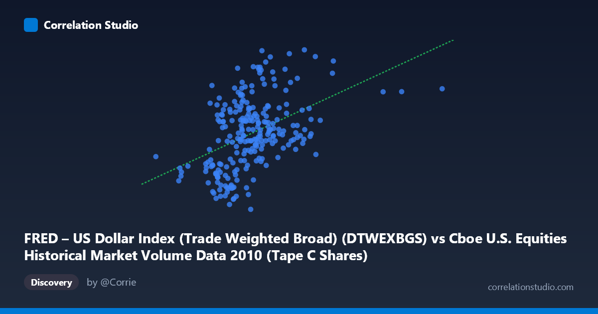
FRED – US Dollar Index (Trade Weighted Broad) (DTWEXBGS) vs Cboe U.S. Equities Historical Market Volume Data 2010 (Tape C Shares)
- Pearson correlation (r)
- 0.4445
- Spearman correlation
- 0.4467
- p-value
- 0
- Sample size (n)
- 245
- 95% confidence interval
- 0.338 to 0.5398
- Granger causality
- None
- Granger optimal lag
- 1
AI analysis
Scatterplot Analysis: US Dollar Index vs. Cboe Tape C Share Volume (2010)
Relationship Overview
The scatterplot reveals a positive relationship between the Trade-Weighted Broad US Dollar Index (X-axis) and Cboe Tape C share volume (Y-axis) across 245 trading days in 2010. As the dollar index increases, Tape C share volume tends to rise modestly, consistent with the fitted regression line (y = 1.84×10⁻⁸x + 89.91). However, the relationship is far from tight — the scatter around the regression line is substantial, indicating that many days with similar dollar index values produce widely varying share volumes, and vice versa. The visual impression is one of a broad, diffuse cloud with a gentle upward tilt rather than a well-defined linear trend.
Correlation Strength and Statistical Interpretation
The Pearson correlation of r = 0.4445 indicates a moderate positive association, but the explanatory power is limited: R² = 0.1976, meaning the dollar index accounts for roughly 20% of the variance in Tape C share volume, leaving 80% unexplained by this variable alone. The 95% confidence interval for r [0.338, 0.540] is meaningfully above zero and excludes it entirely, and the p-value of 2.74×10⁻¹³ confirms the relationship is highly statistically significant given the population of N = 3,302. However, statistical significance here is partially a function of sample size — practical significance remains modest. Critically, the Granger causality tests show no significant directional predictive relationship in either direction: X→Y yields F = 0.709 (p = 0.401) and Y→X yields F = 3.398 (p = 0.067), both failing conventional thresholds. This means the dollar index does not temporally predict future Tape C volume, nor does volume predict the dollar index, cautioning strongly against any causal interpretation.
Notable Patterns, Clusters, and Outliers
Several structural features stand out in the scatterplot. The bulk of observations cluster between approximately 120M–220M on the X-axis and 90–95 on the Y-axis, forming a dense central mass. There appear to be two or three high-Y outliers (Y 97, including values near 97.34, 97.50, 97.55) that sit well above the main cluster — these may correspond to unusual high-volume days coinciding with a stronger dollar, but they exert disproportionate influence on the regression slope. On the low end, a small number of observations with X values below ~100M (e.g., the point near 74M, 91.20) sit isolated from the main cluster, suggesting either low-liquidity days or data anomalies. There is also a notable spread in Y values (88.98–97.55) at similar X values, particularly in the 150M–220M range, reinforcing the weak predictive utility of X alone.
Confounding Factors and Caveats
Several important caveats apply. First, both variables are time-series observed over the same calendar year (2010), meaning their correlation may be partially driven by shared temporal trends — for instance, both could be responding to macroeconomic events (post-GFC recovery, Fed policy, sovereign debt concerns in Europe) rather than directly influencing each other. Second, Tape C volume specifically captures one tape segment of U.S. equities, which may not represent broader market activity uniformly. Third, the dollar index is a broad trade-weighted measure not specifically designed as a market microstructure variable, so any mechanistic link requires careful theoretical justification. Fourth, the presence of high-leverage outliers in the upper-right region may be inflating r beyond what the bulk of the data supports. Finally, the axis labels appear swapped between the dataset descriptions (X is labeled as the dollar index but described under the equities dataset), which warrants verification of data alignment before drawing conclusions.
Actionable Insights and Further Investigation
Despite the caveats, the moderate positive correlation and high statistical significance suggest this relationship warrants further exploration rather than dismissal. Recommended next steps include: (1) conducting a rolling-window correlation analysis across the year to determine whether the relationship is stable or concentrated in specific market regimes; (2) testing whether lagged dollar index values beyond lag-1 (the Granger test only examined one period) show stronger predictive power for volume; (3) decomposing both series (detrending and seasonal adjustment) to isolate whether the correlation survives removal of shared time trends; (4) incorporating additional control variables such as VIX (volatility), S&P 500 returns, or Fed announcement dates to assess how much of the 80% unexplained variance can be recovered; and (5) verifying the axis/dataset mapping to ensure the variables are correctly assigned, given the apparent label inconsistency in the metadata.
X dataset: Cboe U.S. Equities Historical Market Volume Data 2010
Y dataset: FRED – US Dollar Index (Trade Weighted Broad)
Part of experiment: Daily - Cboe U.S. Equities Historical Market Volume Data 2010 vs FRED – US Dollar Index (Trade Weighted Broad)