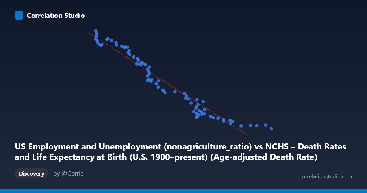
US Employment and Unemployment (nonagriculture_ratio) vs NCHS – Death Rates and Life Expectancy at Birth (U.S. 1900–present) (Age-adjusted Death Rate)
- Pearson correlation (r)
- -0.9712
- Spearman correlation
- -0.9874
- p-value
- 0
- Sample size (n)
- 78
- 95% confidence interval
- -0.9816 to -0.9551
- Granger causality
- None
- Granger optimal lag
- 10
AI analysis
Analysis: Non-Agricultural Employment Ratio vs. Age-Adjusted Death Rate (1941–2018)
Relationship Overview
The scatterplot reveals a strikingly strong negative relationship between the U.S. non-agricultural employment ratio and the age-adjusted death rate. As the share of employment in non-agricultural sectors increases (ranging from roughly 777 to 1,830 units on the X-axis), the age-adjusted death rate falls dramatically — from over 150,000 down to approximately 41,250. The linear regression equation (y = -122.73x + 241,061) quantifies this: for every one-unit increase in the non-agricultural employment ratio, the death rate is predicted to decline by roughly 123 units. The data points trace a remarkably tight, downward-sloping band, suggesting that both variables have been moving in consistent, near-monotonic trends over the 77-year observation window — a hallmark of two time-series variables that are each independently trending over time.
Correlation Strength and Statistical Framing
The Pearson correlation of r = -0.9712 is exceptionally strong, and the R² of 0.9433 means that ~94.3% of the variance in age-adjusted death rates is statistically explained by variation in the non-agricultural employment ratio within this sample. The 95% confidence interval for r is tight at [-0.9816, -0.9551], and the p-value is effectively zero — leaving no ambiguity about statistical significance. However, the Granger causality results complicate the causal picture considerably: neither direction (X→Y nor Y→X) reaches significance (F = 1.63, p = 0.126 and F = 1.69, p = 0.112, respectively, at optimal lag 10). This means that, despite the extraordinary correlation, neither variable demonstrably predicts the other beyond what each predicts about itself over time. This is a critical distinction: the correlation reflects shared temporal drift, not necessarily a directional causal mechanism.
Notable Patterns, Clusters, and Outliers
Several features stand out in the scatter. A dense cluster appears in the lower-left region (X ≈ 776–900, Y ≈ 135,000–155,000), corresponding to earlier decades (likely 1940s–1950s) when death rates were high and non-agricultural employment was lower. A second loose cluster occupies the upper-right area (X ≈ 1,500–1,830, Y ≈ 41,250–55,000), representing recent decades with lower mortality and higher non-agricultural employment. The relationship appears slightly non-linear — the rate of mortality decline appears to decelerate at higher employment ratios, hinting at a possible exponential or power-law decay rather than a purely linear one. A few points, such as (1830.38, 41,250) and (776.72, 153,336), sit at the distributional extremes but remain well within the general trend, suggesting no dramatic outliers.
Confounding Factors and Caveats
This correlation is almost certainly driven primarily by shared secular time trends rather than a direct causal relationship between employment structure and mortality. Both variables trend strongly over time: death rates have fallen due to medical advances, public health improvements, sanitation, and lifestyle changes, while non-agricultural employment ratios have risen due to industrialization, urbanization, and the structural shift toward service economies. This creates spurious correlation — a textbook case where two unrelated-in-mechanism variables appear tightly linked because they are both functions of time. The failure of Granger causality to establish predictive directionality at any lag (up to 10 periods) strongly supports this interpretation. Additional confounders include GDP growth, healthcare spending, demographic shifts (aging population), and technological change — all of which co-evolved with both variables across this period.
Actionable Insights and Further Investigation
Despite the spurious-correlation caveat, these findings are not without value. Researchers should detrend both series (e.g., via first-differencing or HP filtering) before re-examining correlation, which would strip out the shared time trend and reveal whether short-term fluctuations in employment structure genuinely co-move with mortality changes. It would also be valuable to disaggregate by subgroup — race, sex, and cause of death — since the NCHS dataset supports this and occupational mortality risk varies substantially across demographic lines. Testing non-linear specifications (logarithmic or exponential regression) could improve model fit given the apparent curvature. Finally, a multivariate analysis incorporating healthcare access, income inequality (Gini coefficient), and public health expenditure would help isolate whether employment structure carries any independent signal beyond its role as a proxy for economic modernity.
X dataset: NCHS – Death Rates and Life Expectancy at Birth (U.S. 1900–present)
Y dataset: US Employment and Unemployment
Part of experiment: Yearly - NCHS – Death Rates and Life Expectancy at Birth (U.S. 1900–present) vs US Employment and Unemployment