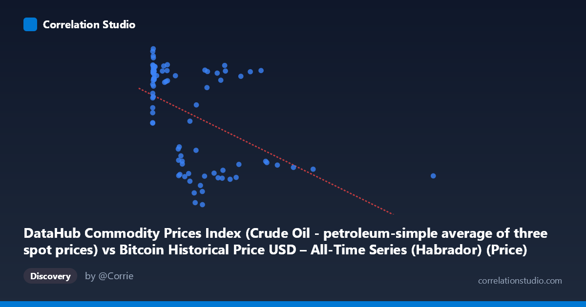
DataHub Commodity Prices Index (Crude Oil - petroleum-simple average of three spot prices) vs Bitcoin Historical Price USD – All-Time Series (Habrador) (Price)
- Pearson correlation (r)
- -0.4787
- Spearman correlation
- -0.4701
- p-value
- 0.000005
- Sample size (n)
- 83
- 95% confidence interval
- -0.6294 to -0.2933
- Granger causality
- None
- Granger optimal lag
- 1
- Time coverage
- 2010-08-01 to 2017-06-01
AI analysis
Analysis: Crude Oil Price Index vs. Bitcoin Historical Price
1. Relationship Overview
The scatterplot reveals a moderate negative, non-linear relationship between crude oil commodity prices (X) and Bitcoin's historical price (Y). The data shows a distinctive pattern: at low X-values (roughly 0–50), Y is highly scattered, ranging from ~76 to ~118, forming a dense cluster on the left side of the chart. As X increases beyond ~100, the point cloud thins out and Y values compress into a lower band (roughly 30–55), with a smaller secondary cluster near X≈600–1000 where Y rebounds to ~100–108. This creates a somewhat bimodal or "L-shaped" scatter rather than a clean linear trend.
2. Strength, Direction, and Statistical Confidence
The correlation coefficient (r = -0.4787) indicates a moderate negative linear association, but r² = 0.2292 shows that only ~23% of the variance in Y is explained by X — meaning over 75% of the variability is driven by other factors. The 95% CI for r [-0.6294, -0.2933] is reasonably tight and entirely negative, and the p-value (4.7×10⁻⁶) confirms this correlation is highly unlikely due to chance. However, statistical significance here reflects a real but weak-to-moderate association, not a strong predictive relationship. Critically, the Granger causality tests show no significant predictive direction in either direction (X→Y: p=0.16; Y→X: p=0.18). This means neither series reliably "leads" the other in time — the correlation is likely coincidental co-movement or driven by a shared external factor, not a causal lag-based relationship.
3. Notable Patterns and Outliers
The most striking feature is the dense vertical band at very low X values (X < 20), where Y spans almost the entire observed range (76–118) — this suggests high Y variance is possible independent of X in this region, weakening the linear fit's practical utility there. A secondary cluster appears at X≈600–1000 with unexpectedly high Y (~100–108), breaking the otherwise declining trend and suggesting non-monotonic behavior — possibly a distinct market regime or time period. The single extreme outlier at X=2452.18 (Y=46.13) sits far from the rest of the data and could disproportionately influence the regression slope. The data is clearly heteroscedastic: variance in Y shrinks as X grows past ~1000.
4. Confounding Factors and Caveats
Since both series are time-based (2010–2017) and neither Granger-causes the other, the correlation is very likely spurious or mediated by a third variable — most plausibly the passage of time itself, macroeconomic cycles, USD strength, or broad market sentiment/liquidity conditions affecting both commodities and crypto simultaneously. Bitcoin's price history is also non-stationary with exponential-like growth phases, and combining it with a mean-reverting commodity index without differencing or detrending can produce artificially inflated correlations. The small paired sample (n=83) relative to the full population (N=449) also raises concerns about sampling representativeness across the full time range.
5. Actionable Insights
Given the lack of Granger causality and modest r², this relationship should not be used for predictive trading or forecasting purposes. Suggested next steps: (a) re-run correlation analysis on returns or differenced/detrended series rather than raw price levels to remove spurious trend-driven correlation; (b) segment the analysis by distinct time periods (e.g., pre-2013 vs. post-2013) to test whether the relationship is regime-dependent, given the visible cluster structure; (c) investigate common macro drivers (USD index, interest rates, overall risk sentiment) as potential confounders; and (d) treat the X=2452 outlier and low-X cluster separately, possibly via robust regression, to assess their influence on the reported slope and r².
X dataset: Bitcoin Historical Price USD – All-Time Series (Habrador)
Y dataset: DataHub Commodity Prices Index
Part of experiment: Bitcoin - Bitcoin Historical Price USD – All-Time Series (Habrador) vs DataHub Commodity Prices Index