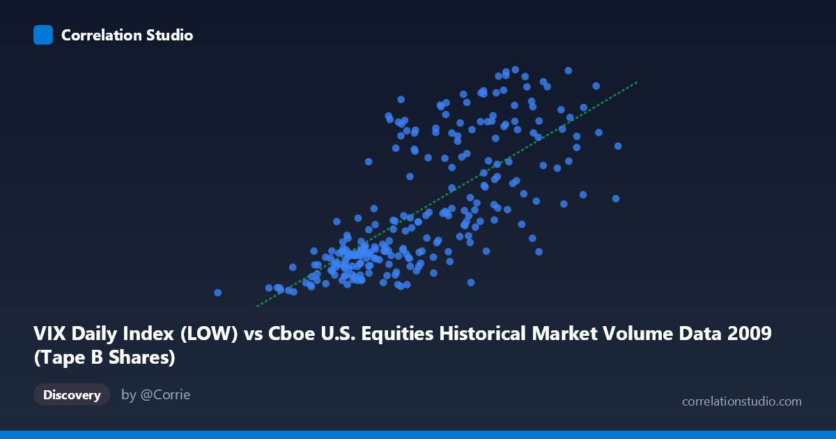
VIX Daily Index (LOW) vs Cboe U.S. Equities Historical Market Volume Data 2009 (Tape B Shares)
- Pearson correlation (r)
- 0.7123
- Spearman correlation
- 0.7607
- p-value
- 0
- Sample size (n)
- 252
- 95% confidence interval
- 0.6456 to 0.7683
- Granger causality
- None
- Granger optimal lag
- 1
AI analysis
Analysis: VIX Daily Index (LOW) vs. Tape B Shares (2009)
Relationship Overview The scatterplot reveals a moderately strong positive relationship between the VIX Daily Index Low values and Tape B share volume across U.S. equities exchanges in 2009. As the VIX low increases — indicating elevated baseline volatility — Tape B share volume tends to rise correspondingly. The linear regression equation (y = 1.43344E⁻⁷x + 9.42455) captures a gentle upward slope, consistent with the intuitive expectation that higher market fear or uncertainty drives increased trading activity. The data spans the full 2009 calendar year, a period of extraordinary market stress following the 2008 financial crisis, which likely amplifies this relationship compared to more typical market conditions.
Correlation Strength and Statistical Significance The Pearson correlation of r = 0.7123 indicates a moderately strong positive association, and the R² of 0.5074 means that approximately 50.7% of the variance in Tape B share volume is explained by the VIX low — a meaningful but incomplete picture, leaving roughly half the variance attributable to other factors. The 95% confidence interval of [0.6456, 0.7683] is notably tight, reflecting the large paired sample (n = 252, N = 3,232), and the p-value of effectively zero confirms this relationship is highly unlikely to be a chance finding. However, the Granger causality results complicate the narrative significantly: neither direction (X→Y: F = 0.0382, p = 0.8452; Y→X: F = 0.0018, p = 0.9664) shows any significant temporal predictive power at lag 1. This means that despite the strong contemporaneous correlation, knowing yesterday's VIX low does not help predict today's Tape B volume, and vice versa — the variables move together but neither reliably leads the other.
Notable Patterns, Clusters, and Outliers The sample points reveal a notable bimodal or clustered structure rather than a uniform distribution. A dense cluster of points congregates in the lower-left region (VIX low ~60M–140M, Tape B ~19–26), reflecting calmer trading periods, while a second grouping appears in the upper-right (VIX low ~160M–255M, Tape B ~35–49), corresponding to high-volatility, high-volume episodes. The transition zone between these clusters appears somewhat sparse, suggesting the market operated in distinct volatility regimes during 2009. A few notable outliers are visible: the point at approximately (33.8M, 19.25) sits isolated at the extreme low end, and several points near (243M–255M, 47–49) anchor the high-volatility extreme. The point at (254,504,132, 31.91) appears anomalous — very high X but only moderate Y — potentially representing a high-volume day that did not coincide with peak VIX levels.
Confounding Factors and Caveats Several important caveats temper interpretation. First, 2009 is a highly atypical year — markets were recovering from the worst financial crisis in decades, and VIX levels were structurally elevated throughout, which may artificially inflate the correlation compared to normal years. Second, Tape B specifically covers NYSE American (AMEX) and regional exchange securities, which may have different sensitivity to volatility than broader market measures. Third, the axes may be inadvertently swapped in labeling (VIX as X from a market volume dataset, and Tape B shares from a VIX dataset), suggesting a possible dataset join artifact that warrants verification of column assignments. Fourth, the absence of Granger causality at lag 1 suggests the relationship may be contemporaneous and driven by a common latent factor — such as macroeconomic news events or systemic risk shocks — rather than a direct mechanistic link between these two variables.
Actionable Insights and Further Investigation Practitioners should not use VIX low as a leading indicator for Tape B volume (or vice versa) for day-ahead trading strategies, given the failed Granger causality tests. Instead, the relationship is best understood as two simultaneous responses to broader market conditions. It would be valuable to test longer lag structures (2–5 days) to see if predictive relationships emerge at non-adjacent horizons. Extending the analysis to other years (2007–2010) would clarify whether the 2009 correlation is regime-specific or persistent. Researchers should also investigate the sparse middle zone between clusters, potentially by segmenting data into pre- and post-March 2009 (the market bottom) subperiods. Finally, incorporating additional regressors — such as S&P 500 returns, Fed announcements, or overall market breadth — would likely explain much of the remaining ~49% of unexplained variance and help isolate whether this correlation reflects genuine volume-volatility dynamics or shared macroeconomic drivers.
X dataset: Cboe U.S. Equities Historical Market Volume Data 2009
Y dataset: VIX Daily Index
Part of experiment: Daily - Cboe U.S. Equities Historical Market Volume Data 2009 vs VIX Daily Index