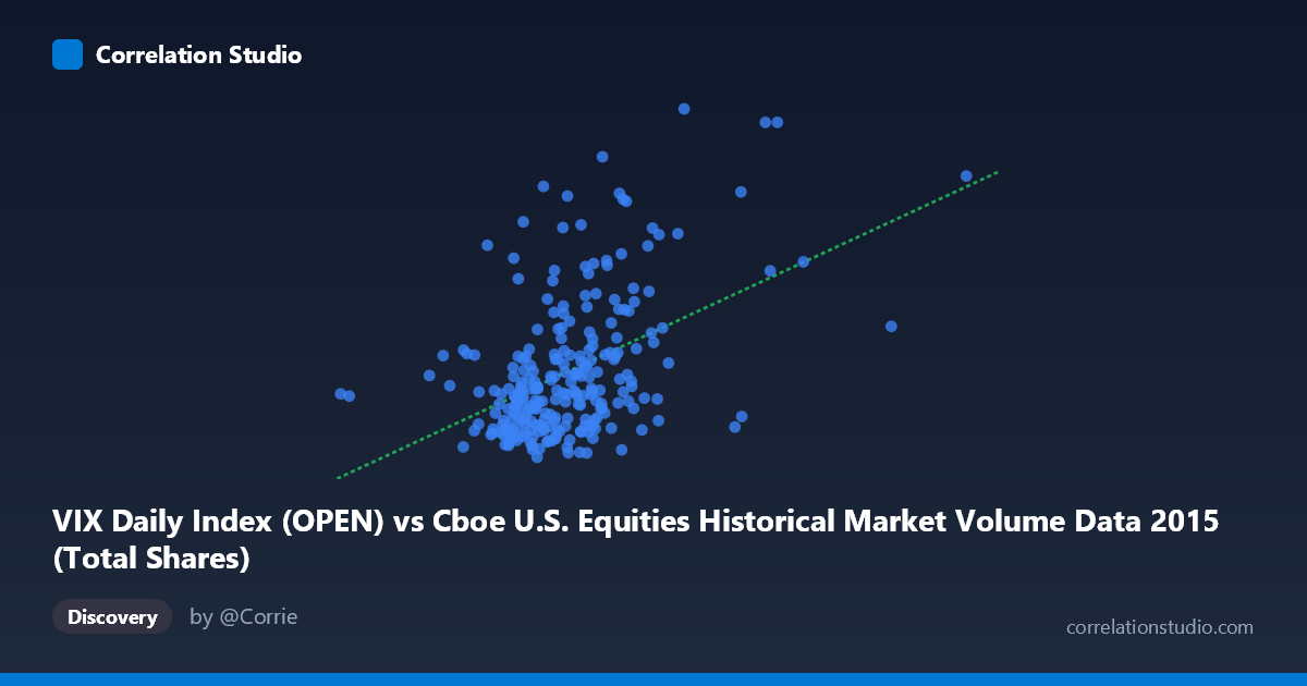
VIX Daily Index (OPEN) vs Cboe U.S. Equities Historical Market Volume Data 2015 (Total Shares)
- Pearson correlation (r)
- 0.4632
- Spearman correlation
- 0.3992
- p-value
- 0
- Sample size (n)
- 252
- 95% confidence interval
- 0.3603 to 0.555
- Granger causality
- None
- Granger optimal lag
- 1
AI analysis
Scatterplot Analysis: VIX Daily Index (Open) vs. Total Shares Traded (2015)
Overall Relationship The scatterplot reveals a moderate positive relationship between the VIX Daily Index opening values and total shares traded on U.S. equities exchanges throughout 2015. As VIX levels rise — indicating greater market fear or uncertainty — trading volume in total shares tends to increase as well. The linear regression equation (y = 1.896E-08x + 6.699) confirms this upward slope, meaning that for every unit increase in VIX open, total shares traded increases modestly. This is an intuitive finding: elevated volatility typically drives heightened market participation as investors react to rapidly changing conditions, either repositioning portfolios or executing hedging strategies.
Correlation Strength and Statistical Significance The Pearson correlation of r = 0.4632 indicates a moderate positive association, but the coefficient of determination r² = 0.2146 is the more sobering figure — it means that VIX open values explain only about 21.5% of the variance in total shares traded, leaving roughly 78.5% attributable to other factors entirely. The 95% confidence interval of [0.3603, 0.5550] is reasonably tight and does not include zero, and the p-value of 8.216E-15 confirms the relationship is highly statistically significant given the sample of 252 paired observations drawn from a population of 3,302. However, statistical significance here is partly a function of sample size — the effect, while real, is far from deterministic. Critically, the Granger causality tests show no significant directional predictive relationship in either direction (X→Y: F=0.0715, p=0.7894; Y→X: F=0.0174, p=0.8951), meaning that knowing yesterday's VIX does not help predict today's volume, and vice versa. The relationship is contemporaneous rather than temporally predictive.
Notable Patterns, Clusters, and Outliers The sample points reveal a few distinct features worth highlighting. The bulk of observations cluster in a relatively compact zone — VIX values roughly between 11–20 paired with share volumes in the 400–600 million range — forming a dense core that anchors the regression line. However, there are notable high-leverage outliers in the upper-right quadrant: points such as (808M shares, VIX ~31.13) and (815M shares, VIX ~22.55) stand out considerably from the main cluster and likely correspond to the August 2015 market selloff, when volatility spiked sharply and volume surged. There also appears to be a non-linear element to the relationship — at moderate VIX levels the data is diffuse and weakly correlated, while the relationship tightens and strengthens at extreme VIX values. This suggests a possible threshold effect where volume-volatility coupling only becomes pronounced during stress events.
Confounding Factors and Caveats Several important caveats apply. First, both variables are likely driven by common underlying macro shocks — events like the China slowdown fears or Federal Reserve rate uncertainty in 2015 could simultaneously spike VIX and drive trading volume, creating a spurious or inflated correlation. Second, day-of-week and seasonal effects in equity trading volumes are well-documented and not controlled for here. Third, the dataset covers only a single calendar year (2015), which includes at least one major volatility regime shift; results may not generalize across different market environments. Fourth, the axis labels appear swapped relative to conventional analysis (VIX is plotted on X, volume on Y), which is appropriate for regression purposes but note that causal intuition should run both ways given the Granger null result. Finally, the linear model may be underfitting a relationship that is better described by a log or power function, given the apparent heteroskedasticity (wider spread at lower VIX levels).
Actionable Insights and Further Investigation Practitioners should resist treating VIX as a reliable day-ahead volume predictor given the failed Granger tests — the relationship is concurrent, not leading. For trading desks or market microstructure analysts, this suggests that real-time VIX monitoring is more useful than VIX-based volume forecasting models. Further investigation should include: (1) segmenting the data by volatility regime (e.g., VIX < 15, 15–20, 20) to test whether the correlation strengthens materially during stress periods; (2) adding lagged macro variables (e.g., S&P 500 returns, credit spreads) to build a more complete volume model; (3) extending the time series across multiple years to test whether the 2015 relationship holds structurally; and (4) applying a log-linear or spline regression to better capture any threshold nonlinearity visible in the upper tail of the distribution.
X dataset: Cboe U.S. Equities Historical Market Volume Data 2015
Y dataset: VIX Daily Index
Part of experiment: Daily - Cboe U.S. Equities Historical Market Volume Data 2015 vs VIX Daily Index