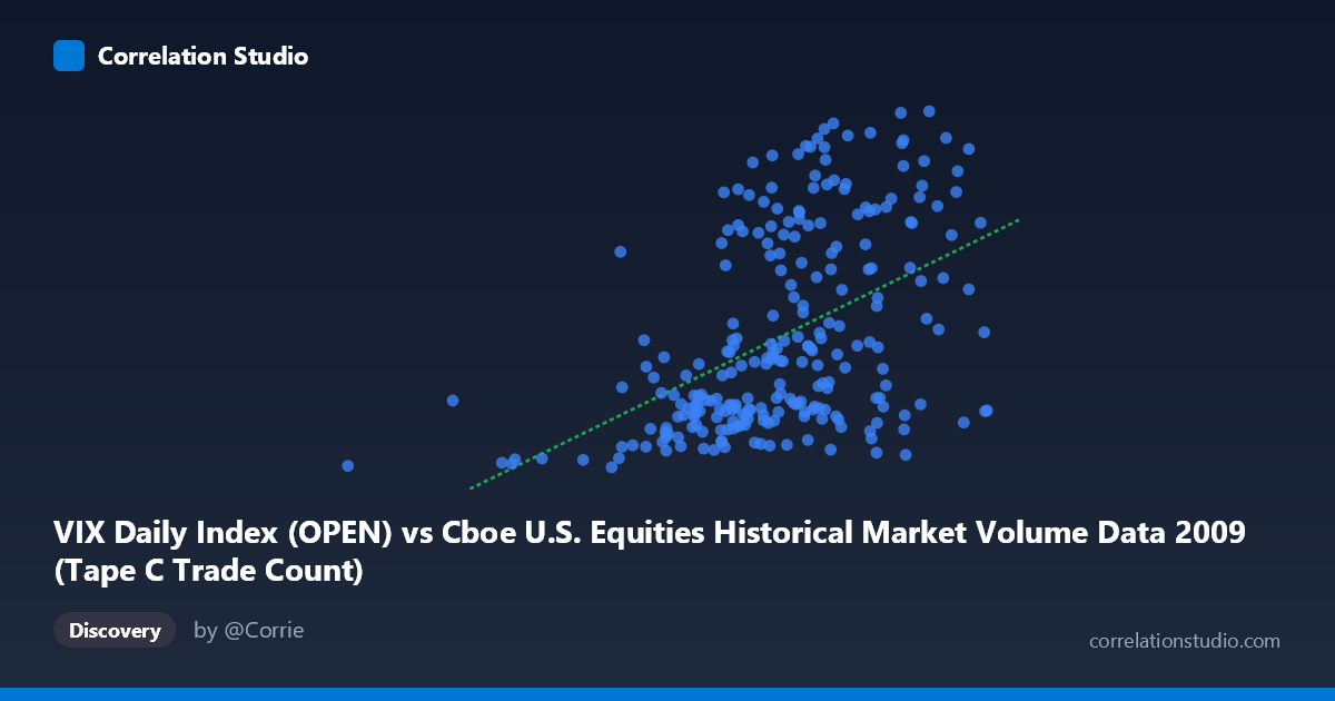
VIX Daily Index (OPEN) vs Cboe U.S. Equities Historical Market Volume Data 2009 (Tape C Trade Count)
- Pearson correlation (r)
- 0.478
- Spearman correlation
- 0.5036
- p-value
- 0
- Sample size (n)
- 252
- 95% confidence interval
- 0.3767 to 0.568
- Granger causality
- None
- Granger optimal lag
- 1
AI analysis
Scatterplot Analysis: VIX Open vs. Tape C Trade Count (2009)
Relationship Overview The scatterplot reveals a moderate positive relationship between the Cboe VIX Daily Index (Open) on the X-axis and the Tape C Trade Count on the Y-axis across 252 trading days in 2009. As the VIX open value increases — indicating rising market volatility expectations — Tape C trade counts tend to rise as well. This is intuitively consistent with market microstructure theory: heightened volatility typically spurs increased trading activity as investors reposition, hedge, or react to uncertainty. The linear regression equation (y = 4.39462E-05x + 3.8015) confirms a positive slope, though the modest coefficient reflects the scale difference between the two variables.
Correlation Strength and Statistical Significance The Pearson correlation of r = 0.478 indicates a moderate positive association. More importantly, the R² of 0.2285 means that only about 22.9% of the variance in Tape C trade counts is explained by VIX open levels — leaving roughly 77% attributable to other factors. The 95% confidence interval of [0.377, 0.568] is reasonably tight and does not cross zero, and the p-value of 8.88E-16 is overwhelmingly significant given the sample of 252 paired observations drawn from a population of 3,232. However, statistical significance here is partly a function of sample size; the practical magnitude of the relationship is moderate at best. Critically, Granger causality tests show no significant predictive direction in either direction (X→Y: F = 0.583, p = 0.446; Y→X: F = 0.0001, p = 0.993), meaning that past VIX values do not reliably predict future trade counts, and vice versa, at a one-period lag. This substantially limits any operational forecasting value of the correlation.
Notable Patterns, Clusters, and Outliers The scatterplot displays several visually distinct features. There appears to be a dense cluster of points at lower VIX values (roughly 185,000–600,000 on the X-axis) with relatively low trade counts (20–30 range), suggesting that during calmer volatility regimes, trading activity in Tape C was subdued and consistent. A second, more dispersed cluster emerges at higher VIX levels, where trade counts span a much wider range (25–52), indicating increased variance at higher volatility — a classic sign of heteroscedasticity. Several potential outliers are visible at the upper extremes: points such as (185,886, 19.67) at the far lower-left and (848,554 range) at the upper-right represent boundary conditions that may disproportionately influence the regression slope. The non-uniform spread across the X-axis range also suggests the data may not be entirely linearly structured.
Confounding Factors and Interpretive Caveats Several important caveats temper interpretation. First, the axis labels appear transposed in the dataset metadata — Tape C Trade Count is listed as originating from the VIX dataset and vice versa, which warrants verification before drawing firm conclusions. Second, 2009 was an extraordinary market year encompassing the tail of the global financial crisis and a major recovery, meaning regime shifts within the year (crisis vs. recovery periods) could be generating the correlation spuriously through a shared time trend rather than a direct functional relationship. Third, Tape C specifically covers NYSE Arca-listed securities, so this reflects a subset of market activity rather than aggregate U.S. equity trading. Finally, the absence of Granger causality at lag-1 suggests the relationship may be contemporaneous rather than predictive, possibly driven by a common underlying factor such as macroeconomic news events.
Actionable Insights and Further Investigation Given the moderate correlation and lack of Granger causality, practitioners should avoid using VIX open levels as a standalone leading indicator for Tape C trade volume. Instead, several follow-up analyses are warranted: (1) Segment the data by pre- and post-March 2009 (market trough) to test whether the correlation is regime-dependent; (2) Test non-linear models (e.g., polynomial or log-log regression) given the apparent heteroscedasticity and potential floor effects at low VIX values; (3) Introduce lagged variables beyond one period and test multivariate Granger causality with controls for broader market volume; (4) Cross-validate against Tape A and Tape B trade counts to determine whether this relationship is specific to Tape C or systemic; and (5) Investigate whether VIX changes (rather than levels) correlate more strongly with trade count changes, which may better capture the reactive nature of trading behavior.
X dataset: Cboe U.S. Equities Historical Market Volume Data 2009
Y dataset: VIX Daily Index
Part of experiment: Daily - Cboe U.S. Equities Historical Market Volume Data 2009 vs VIX Daily Index