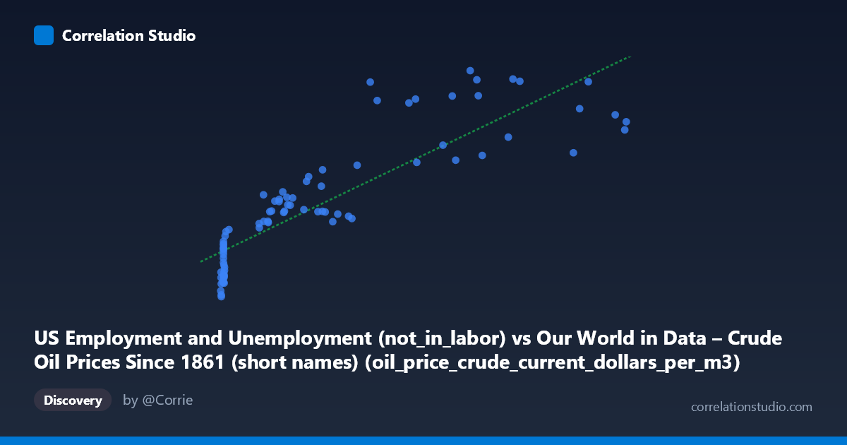
US Employment and Unemployment (not_in_labor) vs Our World in Data – Crude Oil Prices Since 1861 (short names) (oil_price_crude_current_dollars_per_m3)
- Pearson correlation (r)
- 0.8673
- Spearman correlation
- 0.9135
- p-value
- 0
- Sample size (n)
- 85
- 95% confidence interval
- 0.8025 to 0.9119
- Granger causality
- None
- Granger optimal lag
- 10
- Time coverage
- 1941-01-01 to 2025-01-01
- Recomputed on refreshed data
- 2026-10-09 (r was 0.8662)
AI analysis
Analysis: US Not-in-Labor-Force vs. Crude Oil Prices (1941–2024)
1. Overall Relationship The scatterplot reveals a moderately strong positive association between the number of Americans not in the labor force and crude oil prices (in current dollars per cubic meter). As oil prices rise, the not-in-labor-force population also tends to be higher. The linear regression equation (y = 77.82x + 50,771.7) indicates that for every one-unit increase in oil price, approximately 78 more people are counted as not participating in the labor force — though, critically, this arithmetic relationship almost certainly reflects shared historical trends rather than a direct mechanism.
2. Correlation Strength, Uncertainty, and Causality The correlation coefficient (r = 0.866) is strong, and the R² of 0.750 means that roughly 75% of the variance in the not-in-labor-force count is statistically "explained" by oil prices in a purely linear sense. The 95% confidence interval for r is [0.80, 0.91], indicating this is a robustly estimated relationship with relatively narrow uncertainty bounds, and the p-value of essentially zero confirms it is highly unlikely to be a chance finding given the sample size (n = 84). However, the Granger causality results decisively undercut any causal interpretation: neither direction (X→Y nor Y→X) shows significant temporal predictive power (F ≈ 0.67, p ≈ 0.75 in both directions, even at an optimal lag of 10 periods). This means that knowing past oil prices does not help predict future labor force non-participation beyond what is already known, and vice versa. The correlation is real, but it is almost certainly spurious in the causal sense.
3. Patterns, Clusters, and Outliers The scatterplot exhibits two visually distinct clusters. A dense cluster at low X values (roughly X < 50, Y between ~38,000–58,000) corresponds to the mid-20th century era of cheap oil and a smaller, younger US population. A second, more dispersed cluster spans higher oil prices (X = 100–700+) and higher labor-force-non-participation counts (Y = 60,000–100,000+), reflecting the post-1970s through 2020s period. Several notable outliers appear at high Y values relative to X — points near (263, 99,587), (507, 100,465), and (446, 100,241) — which likely correspond to pandemic-era years (2020–2021) when labor force withdrawal spiked dramatically while oil prices were simultaneously volatile. Points like (699, 86,001) and (702, 88,310) sit at very high X but relatively moderate Y, suggesting oil price spikes (e.g., post-Ukraine war 2022) without a proportional labor force response.
4. Confounding Factors and Caveats This correlation is a textbook example of two variables jointly driven by a third factor: time. Both crude oil prices and the not-in-labor-force population have risen substantially since the 1940s — oil due to depletion, geopolitics, and inflation; labor force non-participation due to US population growth, aging Baby Boomers, increased college enrollment, and rising female participation followed by retirement waves. Nominal (non-inflation-adjusted) oil prices compound the problem, as inflation alone inflates both series over eight decades. The dataset labels themselves appear transposed (the axis notes describe each variable as belonging to the other's dataset), which warrants verification of data provenance before drawing any conclusions. Additionally, the 10-period optimal lag in the Granger test spans a decade, making any lagged relationship economically implausible in a direct mechanistic sense.
5. Actionable Insights and Further Investigation Given the spurious nature of this correlation, analysts should detrend both series (e.g., using first differences, HP filter, or per-capita normalization) before drawing any inferences. It would be valuable to investigate whether inflation-adjusted oil prices show a similar pattern — if the correlation weakens substantially, it confirms that nominal price inflation is the primary driver. Researchers should also control for population size and age structure in the labor force variable, converting to rates rather than absolute counts. A more theoretically grounded investigation might examine whether oil price shocks specifically (sudden spikes or drops) have short-term effects on labor force withdrawal — using an event-study or structural VAR framework rather than simple bivariate correlation. Finally, the pandemic-era outliers deserve separate treatment, as they represent a regime-change event that may distort long-run parameter estimates.
X dataset: Our World in Data – Crude Oil Prices Since 1861 (short names)
Y dataset: US Employment and Unemployment
Part of experiment: Yearly - Our World in Data – Crude Oil Prices Since 1861 (short names) vs US Employment and Unemployment