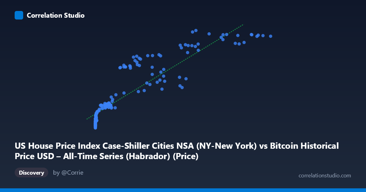
US House Price Index Case-Shiller Cities NSA (NY-New York) vs Bitcoin Historical Price USD – All-Time Series (Habrador) (Price)
- Pearson correlation (r)
- 0.9045
- Spearman correlation
- 0.9603
- p-value
- 0
- Sample size (n)
- 187
- 95% confidence interval
- 0.8744 to 0.9276
- Granger causality
- None
- Granger optimal lag
- 1
AI analysis
Analysis: Bitcoin Price vs. US House Price Index (NY, Case-Shiller)
1. What the Visualization Reveals
The scatterplot shows a strong, positive, non-linear relationship between Bitcoin's historical USD price and the Case-Shiller NY Home Price Index. The data traces a curve that resembles a logarithmic or saturating function: at low Bitcoin prices (under ~$1,000), the HPI clusters tightly in the 157–200 range with very little spread. As Bitcoin price increases into the tens of thousands and beyond, the HPI rises and shows more variance, eventually flattening as it approaches the 300–336 range at the highest Bitcoin prices. This shape suggests the linear R² of 0.818, while high, is partly an artifact of both series trending upward over the same calendar period rather than a tight linear coupling — Bitcoin's price spans nearly 7 orders of magnitude while HPI only spans about 2x, and log-transforming X would likely produce an even better linear fit.
2. Strength, Direction, and Uncertainty
The Pearson r of 0.905 (r² = 0.818) indicates a strong positive linear association, with 81.8% of the variance in Y (HPI) statistically explained by X (Bitcoin price) in a simple linear model. The 95% CI [0.874, 0.928] is tight and doesn't cross zero, and the p-value is effectively 0, so the correlation is not due to chance sampling variability. However, correlation strength should not be mistaken for causal or predictive linkage: the Granger causality tests show no significant predictive direction in either direction (X→Y: p=0.325; Y→X: p=0.202). This is a critical caveat — it means past values of Bitcoin price do not help forecast future HPI values beyond what HPI's own history provides, and vice versa. The relationship is best understood as two series that share a common upward trend over the 2010–2026 window rather than one driving the other in a lead-lag sense.
3. Notable Patterns and Outliers
Several features stand out: - Compression at low X: Nearly all points with X < 1,000 (early Bitcoin history) sit in a narrow HPI band (160–205), reflecting that Bitcoin was a negligible/volatile micro-asset while the housing market moved on its own slower cycle. - Fanning/scatter at mid-to-high X: Between roughly X = 8,000–60,000, HPI values show real spread (e.g., X≈29,000 pairs with Y values ranging from 227 to 294), indicating Bitcoin's sharp boom-bust cycles (2017, 2021 crashes/rallies) occur on a much faster timescale than the steadily-appreciating housing index. - Ceiling effect near the top: At the highest Bitcoin prices (X 85,000), Y values cluster near 330–336, suggesting HPI growth is decelerating/saturating in the visible time window while Bitcoin continues to swing. - No clear discrete clusters or bimodality — the pattern is a continuous, curved sweep rather than separate regimes.
4. Confounding Factors and Caveats
The most important confound is shared time trend: both series generally increased from 2010 to 2026, and both housing prices and Bitcoin were influenced by common macro conditions (near-zero interest rates 2010–2021, quantitative easing, subsequent inflation and rate hikes, speculative risk appetite cycles). This makes the correlation likely spurious in a causal sense — a classic case of two non-stationary trending time series producing high correlation without genuine mechanistic linkage. Additionally, Bitcoin's data spans orders of magnitude while HPI is comparatively smooth and slow-moving (monthly, seasonally-driven), so the pairing conflates a highly volatile asset with a stable index. The unequal variance and scale (Bitcoin stdev ~29,663 vs. HPI stdev ~55) also means the linear fit is dominated by a handful of extreme high-X points.
5. Actionable Insights
- Do not use this correlation for trading or forecasting — the lack of Granger causality confirms neither series leads the other, so using Bitcoin price to predict NY housing prices (or vice versa) is statistically unjustified despite the high r². - De-trend or difference both series (e.g., convert to month-over-month % changes or apply differencing) and recompute correlation; this would reveal whether the relationship survives after removing the shared secular trend, which is a stronger test of genuine co-movement. - Log-transform Bitcoin price before fitting, given its multi-order-of-magnitude range, to check whether a log-linear model fits better and is more interpretable than the raw linear regression. - Introduce control variables — such as CPI/inflation, Fed funds rate, or M2 money supply — to test whether the observed relationship is mediated by a common monetary/macro driver rather than a direct link between crypto and housing markets.
X dataset: Bitcoin Historical Price USD – All-Time Series (Habrador)
Y dataset: US House Price Index Case-Shiller Cities NSA
Part of experiment: Bitcoin - Bitcoin Historical Price USD – All-Time Series (Habrador) vs US House Price Index Case-Shiller Cities NSA