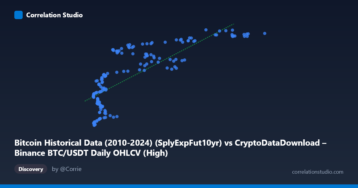
Bitcoin Historical Data (2010-2024) (SplyExpFut10yr) vs CryptoDataDownload – Binance BTC/USDT Daily OHLCV (High)
- Pearson correlation (r)
- 0.802
- Spearman correlation
- 0.8233
- p-value
- 0
- Sample size (n)
- 180
- 95% confidence interval
- 0.7428 to 0.8487
- Granger causality
- None
- Granger optimal lag
- 10
- Time coverage
- 2017-08-20 to 2026-02-02
AI analysis
Analysis of Bitcoin Supply/Futures Metric vs. BTC/USDT Price
1. Relationship Overview
The scatterplot depicts a strong positive, but clearly non-linear (logarithmic-shaped) relationship between the X variable (labeled "SplyExpFut10yr," likely a supply-expansion or futures-related metric) and Y (BTC/USDT daily high price). The data shows a characteristic diminishing-returns curve: Y rises steeply as X increases from ~3,600 to ~20,000, then the rate of increase flattens considerably as X extends out to nearly 119,000. This pattern strongly resembles a log-linear or square-root relationship rather than a straight line, despite the linear fit reporting a positive slope.
2. Strength, Direction, and Statistical Confidence
The Pearson correlation (r = 0.802) indicates a strong positive linear association, with r² = 0.643 meaning the linear model explains about 64% of the variance in Y — leaving over a third of the variability unaccounted for, likely due to the visible curvature. The 95% CI [0.743, 0.849] is reasonably tight given n=180, and the p-value of ~0 confirms the correlation is highly statistically significant and not attributable to chance. However, statistical significance and correlation strength say nothing about causality: the Granger causality tests (X→Y: p=0.441; Y→X: p=0.630) show no significant predictive direction in either direction at the tested lag structure (10 periods). This means neither series reliably "leads" the other in a temporal forecasting sense — the strong contemporaneous correlation is not corroborated by lead-lag predictive power, suggesting both variables may be jointly driven by a common underlying process (e.g., overall market growth/time trend) rather than one causing the other.
3. Notable Patterns and Features
The data clearly clusters into two regimes: a dense cluster of low-X points (roughly X < 25,000) where Y ranges widely from ~20.2M to ~20.7M, and a sparser cluster of high-X points (X 60,000) where Y compresses into a narrow high band (~20.75M–20.83M). This bimodal density plus the flattening tail is classic evidence of a saturating/logarithmic relationship — the linear regression (y = 5.00x + 2.04E7) understates fit quality at the extremes and likely overstates the slope's real-world interpretability. No extreme outliers are apparent, but the low-X cluster shows the most scatter/noise, meaning the relationship is loosest exactly where most data points reside.
4. Confounding Factors and Caveats
A major caveat: X is described as a "10-year supply expansion futures" metric while Y is the daily high price from the same underlying BTC/USDT series — these two "datasets" may not be truly independent, as both are derived from or correlated with Bitcoin's price/market trajectory over time. The shared temporal trend (both variables likely increase somewhat monotonically with calendar time between 2017–2026) is a classic confounder: time itself could be driving apparent correlation, which would also explain why Granger causality fails (a common trend produces contemporaneous correlation without genuine lead-lag predictability). Additionally, n=180 is a sample from a population of 3,212, so sampling method (every-3rd-point selection) could introduce autocorrelation-related bias in variance estimates.
5. Recommendations
Given the visible curvature, refit using a logarithmic or power transformation of X (e.g., y ~ log(x)) to likely improve R² substantially beyond 0.643. Since Granger tests show no predictive direction, this correlation should not be used for forecasting one variable from the other; instead, treat both as co-moving with an underlying market/time trend and consider explicitly detrending (e.g., first-differencing or including a time variable) before re-examining causality. Further investigation should clarify what "SplyExpFut10yr" actually measures and test whether the relationship holds after removing shared trend components, using techniques like cointegration testing given the time-series nature of the data.
X dataset: CryptoDataDownload – Binance BTC/USDT Daily OHLCV
Y dataset: Bitcoin Historical Data (2010-2024)
Part of experiment: Bitcoin - CryptoDataDownload – Binance BTC/USDT Daily OHLCV vs Bitcoin Historical Data (2010-2024)