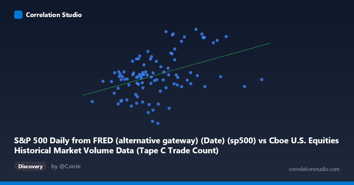
S&P 500 Daily from FRED (alternative gateway) (Date) (sp500) vs Cboe U.S. Equities Historical Market Volume Data (Tape C Trade Count)
- Pearson correlation (r)
- 0.4154
- Spearman correlation
- 0.347
- p-value
- 0.000021
- Sample size (n)
- 98
- 95% confidence interval
- 0.2364 to 0.567
- Granger causality
- None
- Granger optimal lag
- 10
AI analysis
Analysis: S&P 500 Daily Values vs. Cboe Tape C Trade Count
Relationship Overview
The scatterplot reveals a modest positive relationship between S&P 500 index levels (X-axis) and Cboe U.S. Equities Tape C trade counts (Y-axis) over the January–May 2026 period. As S&P 500 values increase, Tape C trade counts tend to rise as well, following the linear regression equation y = 0.000330x + 5868.82. However, the relationship is far from tight — the scatter is considerable across the full X range of roughly 2.58M to 4.34M, suggesting that index level alone is a weak predictor of daily trade activity. The data spans 98 paired observations drawn from a population of 1,980 trading days, making the sample reasonably representative but still subject to seasonal and structural limitations.
Correlation Strength and Statistical Significance
The Pearson correlation of r = 0.4154 indicates a moderate positive association, but the R² of 0.1725 is the more sobering figure: S&P 500 level explains only about 17.3% of the variance in Tape C trade counts, leaving roughly 83% attributable to other factors. The 95% confidence interval for r spans [0.2364, 0.5670], which is meaningfully wide — while the lower bound confirms a real positive relationship, the upper bound suggests it could be substantially stronger or weaker in other periods. The p-value of 2.11×10⁻⁵ confirms strong statistical significance at conventional thresholds, so the correlation is unlikely to be a sampling artifact. Critically, Granger causality tests find no significant temporal predictive direction in either direction (X→Y: F=0.66, p=0.76; Y→X: F=1.10, p=0.37), meaning that even though the two variables co-move to some degree, lagged values of one do not reliably predict the other. This rules out a simple leading-indicator relationship and suggests the correlation is largely contemporaneous and likely driven by shared underlying forces.
Notable Patterns, Clusters, and Outliers
Several features stand out visually. There is a dense cluster of points in the X range of ~2.9M–3.4M with Y values between approximately 6,500–7,200, forming the core of the distribution and anchoring the regression line. A second, sparser upper-right cluster appears around X = 3.5M–3.9M with notably elevated Y values (7,300–7,500), pulling the regression slope upward and suggesting that higher market levels in this period coincided with elevated small-cap or retail trading activity (Tape C covers NASDAQ-listed securities). Several potential outliers are visible: the point near (3,262,293, 6,343.72) shows a very low Y value for its X position, while (3,658,890, 7,501.24) anchors the upper-right extreme. The point at X ≈ 4,341,728 (the rightmost observation) has a surprisingly moderate Y value (~6,882), breaking the upward trend and suggesting the relationship may not hold linearly at extreme market levels.
Confounding Factors and Caveats
Several confounds complicate a causal interpretation. First, both variables are likely driven by common macroeconomic conditions — periods of economic uncertainty or Federal Reserve announcements can simultaneously move index prices and spike trading volumes, creating spurious correlation. Second, Tape C specifically captures NASDAQ-listed securities, which skews toward technology and growth stocks; periods when tech outperforms or underperforms the broader S&P 500 could distort this relationship relative to full-market measures. Third, the five-month window (Jan–May 2026) may capture a structural trend — if markets were broadly rising during this period, both variables would trend upward in tandem without a causal link. The lack of Granger causality at the optimal 10-period lag further cautions against assuming any mechanistic relationship. Finally, the mismatch in dataset labeling (X-axis described as S&P 500 dates but values in millions suggest a volume/notional metric rather than a price index) warrants careful verification of the axis assignments.
Actionable Insights and Further Investigation
Given that only 17% of variance is explained and no Granger causality is detected, practitioners should avoid using S&P 500 level alone as a predictive signal for Tape C trade counts. A more productive direction would be to incorporate volatility measures (VIX), market breadth indicators, or options expiration calendars as additional covariates, since trade counts are often driven by hedging and rebalancing activity rather than directional price levels. It would also be worthwhile to decompose Tape C counts by trade size (retail vs. institutional) to identify which segment drives the correlation. Running the analysis over a longer window (the full 2009–present dataset available) would clarify whether this moderate correlation is a stable structural feature or an artifact of the specific 2026 market regime. Finally, testing non-linear specifications (e.g., quadratic or piecewise regression) could better capture the apparent clustering behavior visible at both low and high X values.
X dataset: Cboe U.S. Equities Historical Market Volume Data
Y dataset: S&P 500 Daily from FRED (alternative gateway) (Date)
Part of experiment: Daily - Cboe U.S. Equities Historical Market Volume Data vs S&P 500 Daily from FRED (alternative gateway) (Date)