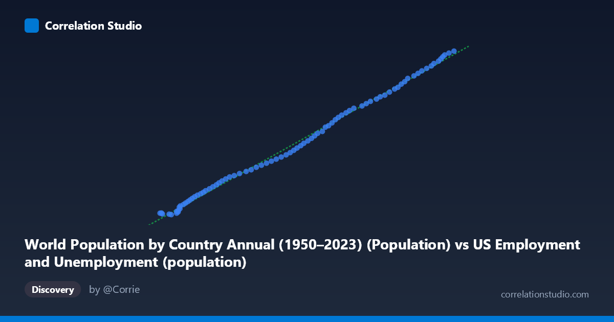
World Population by Country Annual (1950–2023) (Population) vs US Employment and Unemployment (population)
- Pearson correlation (r)
- 0.9983
- Spearman correlation
- 0.9994
- p-value
- 0
- Sample size (n)
- 83
- 95% confidence interval
- 0.9973 to 0.9989
- Granger causality
- None
- Granger optimal lag
- 10
AI analysis
Scatterplot Analysis: US Employment Population vs. World Population
Relationship Overview
The scatterplot reveals a strikingly tight, nearly perfect linear relationship between the US employment population (X-axis, sourced from BLS data) and the world population estimate (Y-axis, from global demographic records) across the 1941–2023 timeframe. The data points form an almost unbroken diagonal line from the lower-left to the upper-right, indicating that as the US civilian population tracked by employment statistics grows, the global population figure rises in near-perfect lockstep. The linear regression equation y = 676.212x − 19,675,300 captures this relationship with extraordinary precision, suggesting both series trend upward together across the 83-year observation window with minimal scatter around the fitted line.
Correlation Strength and Statistical Framing
The correlation coefficient of r = 0.9983 is exceptional, and the coefficient of determination r² = 0.9965 means that 99.65% of the variance in the world population figure is statistically explained by variation in the US employment population series. The 95% confidence interval for r is extremely narrow at [0.9973, 0.9989], confirming that this estimate is highly stable and not an artifact of sampling variability. The p-value of effectively zero leaves no doubt about statistical significance. However, the Granger causality results introduce a critical qualification: neither X→Y (F = 1.53, p = 0.154) nor Y→X (F = 1.58, p = 0.139) shows statistically significant temporal predictive power at any tested lag up to 10 periods. This means that while the two series move together almost perfectly, neither one reliably predicts future movements in the other beyond what baseline trends already explain — a finding that sharply limits any causal interpretation.
Patterns, Clusters, and Outliers
The distribution of points is remarkably uniform along the regression line, with no dramatic outliers, leverage points, or breaks in trend visible across the full range (X: ~93,000–267,000; Y: ~46.4M–163.2M). The data cluster slightly more densely in the lower-left region (earlier decades, smaller populations), with greater spread in the upper-right corresponding to more recent years of rapid population growth. There is no visible heteroscedasticity — the variance around the line appears consistent across the full range — and no evidence of non-linearity, plateau effects, or structural breaks that might suggest regime changes (e.g., post-WWII baby boom, immigration surges, or COVID-era disruptions). This uniformity is itself a notable finding worth scrutinizing.
Confounding Factors and Caveats
The near-perfect correlation is almost certainly a classic case of spurious correlation driven by shared secular time trends — both series simply grow over time as a function of global and national demographic expansion across the 20th and early 21st centuries. Any two steadily increasing time series measured over 80+ years will tend to correlate strongly regardless of any meaningful causal connection. The fact that the X-axis variable is labeled as coming from a "World Population by Country" dataset while referencing a US employment column — and vice versa — also raises dataset labeling ambiguity that should be clarified before drawing conclusions. Additionally, the optimal Granger lag of 10 periods is relatively long for annual data, and the non-significant causality result reinforces that this correlation reflects parallel demographic trends, not a mechanistic or policy-relevant relationship.
Actionable Insights and Further Investigation
Given the spurious correlation concern, the most important next step is to detrend both series (e.g., using first differences or percentage year-over-year changes) and re-examine the correlation — a genuine relationship should persist even after removing shared time trends, while a spurious one will likely collapse toward zero. Researchers should also verify the dataset column assignments, as the axis labels suggest potential metadata swapping between the two sources. If a genuine relationship is hypothesized — for instance, that US labor force size reflects broader demographic pressures with global implications — partial correlation analyses controlling for calendar year, GDP, or immigration rates would be informative. Finally, segment-level analysis by decade could reveal whether the co-movement is stable or whether certain historical periods (1970s stagflation, 2008 recession, COVID-19) produce meaningful deviations that the aggregate correlation obscures.
X dataset: US Employment and Unemployment
Y dataset: World Population by Country Annual (1950–2023)
Part of experiment: Yearly - US Employment and Unemployment vs World Population by Country Annual (1950–2023)