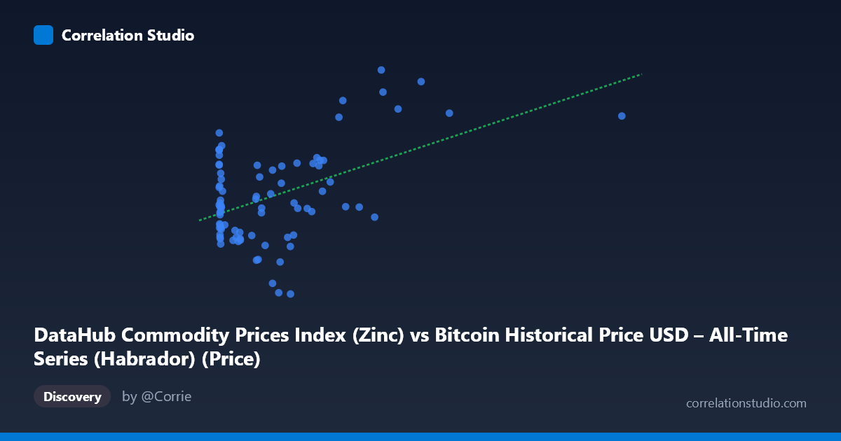
DataHub Commodity Prices Index (Zinc) vs Bitcoin Historical Price USD – All-Time Series (Habrador) (Price)
- Pearson correlation (r)
- 0.4717
- Spearman correlation
- 0.1861
- p-value
- 0.000007
- Sample size (n)
- 83
- 95% confidence interval
- 0.2851 to 0.624
- Granger causality
- None
- Granger optimal lag
- 10
- Time coverage
- 2010-08-01 to 2017-06-01
- Recomputed on refreshed data
- 2026-10-24 (r was 0.4717)
AI analysis
Analysis: Zinc Price Index vs. Bitcoin Historical Price
1. Overview of the Relationship
The scatterplot depicts a moderate positive association between the Zinc commodity price index (X-axis) and Bitcoin price in USD (Y-axis) across 83 paired observations spanning 2010–2017. The data shows a general upward trend — as zinc index values increase, Bitcoin prices tend to rise as well — but the relationship is loose and scattered rather than tight or deterministic. The bulk of observations cluster in the lower-left region (X < 300, Y between 1800–2400), with a sparser tail of higher-X points extending toward the upper right.
2. Strength, Direction, and Statistical Confidence
The correlation coefficient (r = 0.472) indicates a moderate positive linear relationship, but r² = 0.223 reveals that zinc prices explain only about 22% of the variance in Bitcoin prices — leaving roughly 78% attributable to other factors. The 95% confidence interval [0.285, 0.624] is fairly wide, reflecting real uncertainty in the true population correlation strength, though it excludes zero, and the extremely small p-value (6.7×10⁻⁶) confirms the correlation is statistically significant and unlikely due to chance. However, statistical significance here should not be conflated with practical predictive power given the small r². Critically, the Granger causality tests show no significant predictive direction in either direction (X→Y: p=0.704; Y→X: p=0.979), meaning that despite the contemporaneous correlation, neither variable's past values help forecast the other's future values. This strongly suggests the correlation is not causal in a temporal/dynamic sense — it may instead reflect a shared underlying driver (e.g., both assets influenced by general macroeconomic risk sentiment, USD strength, or a coincidental co-trending pattern over 2010–2017).
3. Patterns, Clusters, and Outliers
The data shows a dense cluster of points with X < 50 and Y in the 1800–2400 range — likely corresponding to an early period of low zinc index values coinciding with Bitcoin's earlier, more volatile but bounded price history. A second, more dispersed group appears at higher X values (600–2452) with correspondingly higher Y values (2500–2850), suggestive of a later period when both series were elevated. This bimodal/clustered structure, rather than a smooth continuous cloud, hints that the "correlation" may be substantially driven by two time-block regimes rather than a consistent point-by-point relationship. Notable outliers include a few high-Y points (e.g., ~2845, 2777, 2715) at moderate X values (900–1400), and one extreme X outlier at 2452.18 (Y=2573), which sits far from the main point cloud and could exert leverage on the regression slope.
4. Confounding Factors and Caveats
Since both series are time series (2010–2017) rather than independent cross-sectional samples, the correlation is highly susceptible to spurious trend correlation — two unrelated series that both trend upward over time (Bitcoin's well-known long-term appreciation, and zinc's cyclical recovery post-2015) will show correlation even without any causal link. The lack of Granger causality reinforces this concern. Additionally, sample autocorrelation violates the independence assumption underlying the r and p-value calculations, meaning the true effective sample size is smaller than n=83, and the p-value is likely overstated in significance. No adjustment for inflation, exchange rate effects, or detrending has been applied, and both series may be non-stationary.
5. Recommendations for Further Investigation
Analysts should detrend or difference both series (e.g., using returns/percent changes rather than levels) and re-test correlation and Granger causality to rule out spurious trend-driven association. It would also be valuable to segment the analysis by sub-period (early vs. late cycle) to check whether the relationship is driven by a specific regime rather than a stable structural link. Given the absence of Granger causality, this pair should not be used for predictive trading signals in either direction; instead, treat the correlation as coincidental co-movement, and investigate common macro drivers (USD index, global risk appetite, industrial demand cycles) that might independently explain both series' trends.
X dataset: Bitcoin Historical Price USD – All-Time Series (Habrador)
Y dataset: DataHub Commodity Prices Index
Part of experiment: Bitcoin - Bitcoin Historical Price USD – All-Time Series (Habrador) vs DataHub Commodity Prices Index