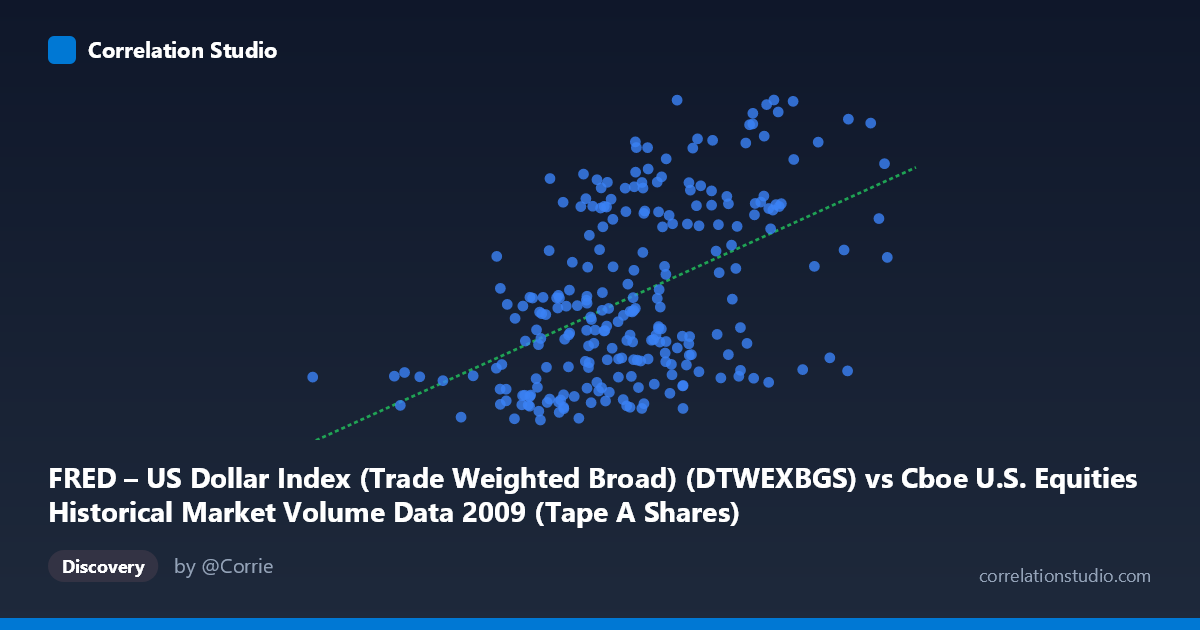
FRED – US Dollar Index (Trade Weighted Broad) (DTWEXBGS) vs Cboe U.S. Equities Historical Market Volume Data 2009 (Tape A Shares)
- Pearson correlation (r)
- 0.4898
- Spearman correlation
- 0.4645
- p-value
- 0
- Sample size (n)
- 248
- 95% confidence interval
- 0.389 to 0.5791
- Granger causality
- None
- Granger optimal lag
- 1
AI analysis
Analysis: US Dollar Index vs. Cboe Equity Market Volume (2009)
Relationship Overview
The scatterplot reveals a modest positive relationship between the Trade Weighted Broad US Dollar Index (X-axis) and Cboe Tape A Share volume (Y-axis) across 248 trading days in 2009. As dollar index values increase — roughly spanning 105 million to 704 million in the index units recorded — share volume tends to drift upward from the low-90s toward the mid-100s range. The linear regression equation (y = 2.07×10⁻⁸x + 87.60) confirms this positive slope, though the relationship is far from deterministic. The visual pattern shows a broad, dispersed cloud of points with a discernible but weak upward trend, suggesting that while the two variables move in the same general direction, many days deviate substantially from the fitted line.
Correlation Strength and Statistical Significance
The Pearson correlation of r = 0.49 indicates a moderate positive association, but the explained variance tells a more sobering story: r² = 0.24, meaning only about 24% of the day-to-day variation in share volume is attributable to dollar index levels. The remaining 76% is driven by other factors entirely. The 95% confidence interval for r ([0.389, 0.579]) is reasonably tight given the sample size of n = 248, and the p-value of 2.22×10⁻¹⁶ confirms the correlation is highly statistically significant — the relationship is almost certainly real rather than a sampling artifact. However, statistical significance should not be mistaken for practical magnitude; with N = 3,232 population-level observations and a large sample, even modest true correlations will register as highly significant. Critically, the Granger causality tests find no significant predictive directionality in either direction (X→Y: F = 0.26, p = 0.61; Y→X: F = 0.006, p = 0.94), meaning neither variable meaningfully predicts the other's next-period movement at a 1-period lag. This firmly limits any causal or forecasting interpretation.
Notable Patterns and Outliers
Several features stand out in the point cloud. There is a visible clustering of observations in the 380–550 million dollar index range paired with volume readings between 91 and 103, forming the dense core of the distribution. However, the right tail of the X distribution (values above 600 million) shows points that span the full vertical range — some reaching the highest volume readings (~104–106) and others sitting near the lowest (~93), which weakens the linear story at extreme values. A handful of potential outliers are visible: one point near (105M, 92.87) is far to the left of the main cluster, likely representing an anomalous early-2009 trading session, and points near (485M, 106) and (590M, 105.5) sit notably above the regression line. The spread of Y values at any given X level is wide — often 10–12 units of volume range for a fixed X band — reinforcing that the relationship is noisy.
Confounding Factors and Caveats
This correlation is subject to several important confounds. 2009 was an extraordinary market year, spanning the tail of the financial crisis, the March 2009 market bottom, and a sharp recovery — structural regime changes that would independently drive both dollar strength and trading volumes in ways that could create spurious correlations. Both variables may be simultaneously responding to a common third driver, such as systemic risk appetite, Federal Reserve policy actions, or global capital flow dynamics, rather than influencing each other directly. The dataset covers only a single calendar year, making it impossible to determine whether this relationship is structurally persistent or period-specific. Additionally, the Granger causality result at lag-1 only tests one-day-ahead predictability; relationships at longer lags (weekly or monthly) may behave differently. The axis labels also appear to be swapped in the dataset metadata (the FRED dollar index is labeled as X but the column description for Y references the dollar index), warranting a careful data audit before drawing conclusions.
Actionable Insights and Further Investigation
Given the moderate but statistically robust correlation with no Granger-causal directionality, practitioners should treat these variables as co-moving indicators of broader market conditions rather than predictors of each other. Several next steps are warranted: (1) Extend the analysis beyond 2009 to test whether the r ≈ 0.49 relationship holds across different market regimes, particularly calm versus stressed periods; (2) Apply partial correlation or multivariate regression controlling for the VIX, S&P 500 returns, and Fed funds rate to isolate the net dollar-volume relationship; (3) Test longer Granger lags (5, 10, 21 days) to see if any predictive signal emerges at weekly or monthly horizons; (4) Investigate whether the relationship is non-linear — a polynomial or spline fit may better capture behavior at the extremes of the dollar index distribution; and (5) Clarify and correct the apparent metadata axis labeling inconsistency to ensure the analytical conclusions are grounded in correctly identified variables.
X dataset: Cboe U.S. Equities Historical Market Volume Data 2009
Y dataset: FRED – US Dollar Index (Trade Weighted Broad)
Part of experiment: Daily - Cboe U.S. Equities Historical Market Volume Data 2009 vs FRED – US Dollar Index (Trade Weighted Broad)