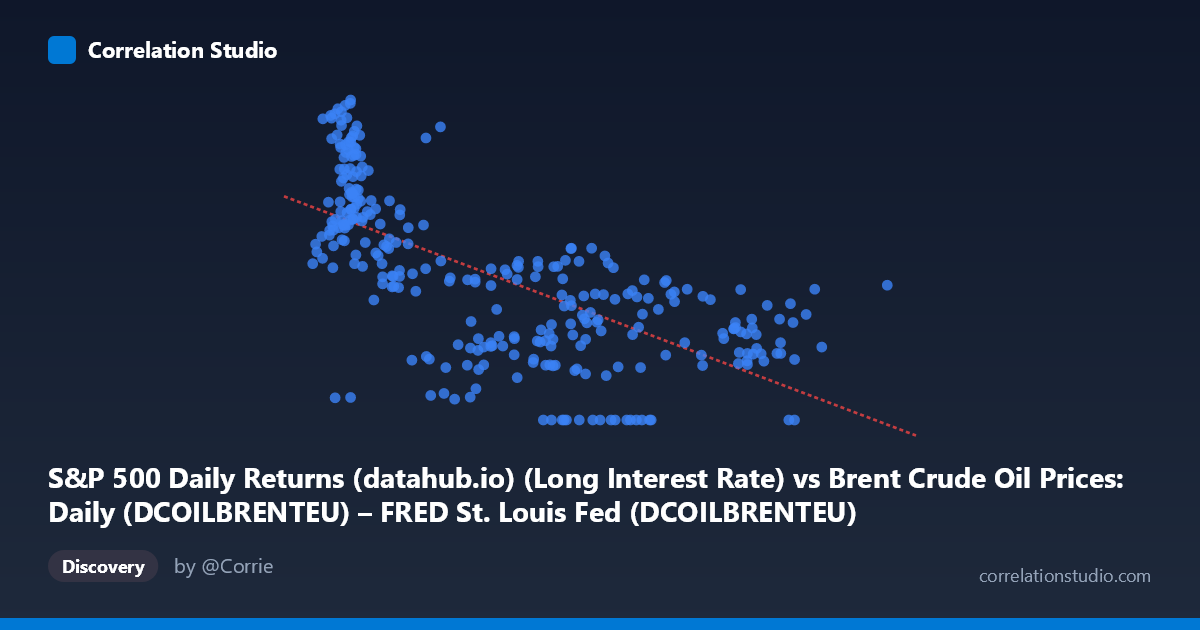
S&P 500 Daily Returns (datahub.io) (Long Interest Rate) vs Brent Crude Oil Prices: Daily (DCOILBRENTEU) – FRED St. Louis Fed (DCOILBRENTEU)
- Pearson correlation (r)
- -0.6753
- Spearman correlation
- -0.7222
- p-value
- 0
- Sample size (n)
- 297
- 95% confidence interval
- -0.7328 to -0.6083
- Granger causality
- None
- Granger optimal lag
- 1
AI analysis
Analysis: Brent Crude Oil Prices vs. S&P 500 Long Interest Rate
Relationship Overview
The scatterplot reveals a moderate negative relationship between the long interest rate associated with S&P 500 data and Brent Crude Oil prices, with higher interest rate values corresponding to lower crude oil prices. The linear regression equation (y = -0.0495x + 6.820) quantifies this inverse slope: for every one-unit increase in the X variable, oil prices decline by approximately $0.05 per barrel on average. The relationship is visually apparent in the data — points clustered at lower X values (roughly 10–40) tend to show Y values between 4–9.5, while points at higher X values (80–140) cluster at Y values between 0–4. This broad directional pattern is consistent throughout the sample, though with considerable scatter around the regression line.
Correlation Strength and Statistical Significance
The Pearson correlation of r = -0.675 indicates a moderate-to-strong negative association, and with r² = 0.456, approximately 45.6% of the variance in Brent crude oil prices is explained by the long interest rate variable. While this is a meaningful explanatory share, it equally implies that 54.4% of variation remains unexplained by this relationship alone. The 95% confidence interval of [-0.733, -0.608] is relatively tight and lies entirely in negative territory, lending strong statistical confidence to the direction of the effect. The p-value of effectively zero, derived from a population of N = 1,865 monthly observations spanning 1987–2026, confirms this is not a chance finding. However, the Granger causality tests complicate the picture significantly: neither direction (X→Y: F = 0.0005, p = 0.983; Y→X: F = 0.728, p = 0.394) shows statistically significant temporal predictive power at a one-period lag. This means that while the variables are correlated in levels, neither reliably predicts future changes in the other — a crucial caveat against any causal interpretation.
Notable Patterns, Clusters, and Outliers
Several structural features stand out in the data. There is a pronounced cluster of high-Y, low-X observations (interest rates below 30, oil prices above 5), which likely corresponds to the post-2008 low-rate environment or early-period data when rates were compressed and energy markets were elevated. Conversely, a second cluster at mid-to-high X values (60–100) shows considerable dispersion in Y, ranging from near zero to nearly 5, suggesting the relationship weakens or becomes noisier at moderate interest rate levels. Zero-valued Y observations appear at multiple X values (e.g., 67.09, 73.63, 84.82, 86.92), which likely represent data artifacts, missing values coded as zero, or true market disruptions rather than genuine oil price readings — these points should be treated as potential outliers. The point at (18.50, 9.52) represents the maximum observed oil-adjusted value and sits somewhat above the regression line, while (115.55, 1.98) and (140.67 range points) anchor the high-X, low-Y tail.
Confounding Factors and Interpretive Caveats
Several important caveats temper this analysis. First, the axis labels appear to be swapped or mislabeled in the metadata — the X-axis is described as "Long Interest Rate" from a Brent Crude dataset, while the Y-axis is labeled as Brent prices from an S&P 500 dataset, suggesting a data pipeline or column-assignment issue that warrants verification before drawing firm conclusions. Second, both interest rates and oil prices are jointly influenced by macroeconomic cycles — recessions, monetary policy regimes, geopolitical shocks, and global demand fluctuations — making it very difficult to isolate a direct bilateral relationship. The 1987–2026 window spans dramatically different monetary regimes (high-rate 1980s, zero-lower-bound 2009–2015, post-COVID tightening), which likely drive structural breaks in the relationship. Third, the monthly aggregation used here may obscure higher-frequency dynamics, and the absence of Granger causality at one lag does not rule out longer-lag predictive relationships.
Actionable Insights and Further Investigation
Given these findings, several analytical steps would add value. First, the zero-valued Y observations should be investigated and likely removed or imputed, as they distort the regression and correlation estimates. Second, regime-based subgroup analysis — segmenting by Federal Reserve policy periods or oil price supercycles — would test whether the r = -0.675 aggregate correlation masks distinct subperiod relationships. Third, a cointegration test (e.g., Engle-Granger or Johansen) would be more appropriate than Granger causality for these likely non-stationary level series, potentially revealing a long-run equilibrium relationship even where short-run predictability is absent. Fourth, extending the Granger analysis to lags of 3, 6, and 12 periods could uncover slower-moving predictive dynamics consistent with monetary policy transmission. Finally, adding control variables — global GDP growth, USD index, OPEC supply decisions — into a multivariate framework would help determine whether the observed correlation is a direct relationship or largely a shared response to common macroeconomic drivers.
X dataset: Brent Crude Oil Prices: Daily (DCOILBRENTEU) – FRED St. Louis Fed
Y dataset: S&P 500 Daily Returns (datahub.io)
Part of experiment: Daily - Brent Crude Oil Prices: Daily (DCOILBRENTEU) – FRED St. Louis Fed vs S&P 500 Daily Returns (datahub.io)