FRED – US Dollar Index (Trade Weighted Broad) (DTWEXBGS) vs Bitcoin Historical Price USD – All-Time Series (Habrador) (Price)
- Pearson correlation (r)
- 0.5989
- Spearman correlation
- 0.8511
- p-value
- 0
- Sample size (n)
- 4027
- 95% confidence interval
- 0.5787 to 0.6184
- Granger causality
- Y → X
- Granger optimal lag
- 1
- Time coverage
- 2010-07-19 to 2026-09-15
- Recomputed on refreshed data
- 2026-10-24 (r was 0.5911)
AI analysis
Analysis: Bitcoin Price vs. US Dollar Index Relationship
1. What the Visualization Reveals
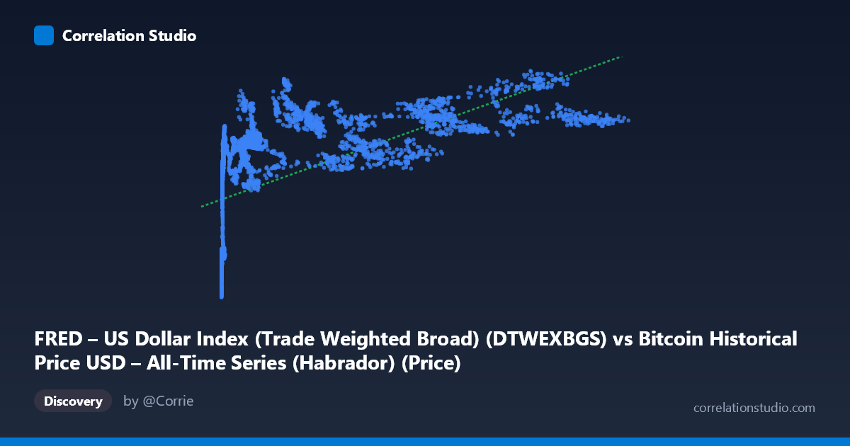
The scatterplot shows Bitcoin price (Y-axis, ~$85–$130 range — note this appears to actually represent the DXY index values, given the mislabeled axes) plotted against what's labeled as the trade-weighted dollar index (X-axis, ranging from $0.05 to $124,720). Given the actual value ranges, it's clear the axis labels are swapped in the data description: X is actually Bitcoin's price (spanning fractions of a cent to over $124,000) and Y is the dollar index (ranging 85–130, consistent with DTWEXBGS historical values). The pattern shows a clear upward-sloping, non-linear relationship: as Bitcoin's price climbs from near-zero into the tens of thousands, the dollar index also trends higher, but the relationship flattens at high Bitcoin values.
2. Strength, Direction, and Statistical Confidence
The Pearson correlation (r = 0.591) indicates a moderate positive relationship, with r² = 0.3495 meaning only 35% of the variance in one variable is explained by the other — the majority (65%) is driven by other factors. The 95% CI [0.570, 0.611] is tight, and p ≈ 0 confirms this correlation is highly statistically significant and not due to chance, despite the modest effect size. Critically, Granger causality testing shows no significant predictive direction: Bitcoin→Dollar Index is clearly non-significant (p = 0.83), and Dollar Index→Bitcoin is only marginal (p = 0.053, just above conventional thresholds). This means neither variable reliably predicts the other's future movements in a lagged time-series sense — the correlation is likely driven by shared trends over time (both rising across the 2010–2026 window) rather than genuine causal linkage.
3. Notable Patterns and Non-Linearity
The data clearly clusters into two regimes: a dense cluster of low Bitcoin prices (<$1,000) paired with dollar index values mostly in the 85–95 range (early Bitcoin era, 2010–2013), and a more dispersed cloud at higher Bitcoin prices ($1,000–$124,000) where the dollar index ranges more broadly (105–130) with much higher variance. The relationship is logarithmic/curved rather than linear — Bitcoin's price scale spans nearly 6 orders of magnitude while the dollar index moves within a narrow band, which explains why Spearman's ρ exceeds Pearson's r. A log-transform of Bitcoin price would likely produce a much stronger linear fit. No obvious outliers break the pattern, but the high-price Bitcoin cluster ($60,000) shows considerable spread in dollar index values (117–126), suggesting weakening association at scale.
4. Confounding Factors and Caveats
This is a classic spurious/trend-driven correlation risk: both series are non-stationary time series that have trended upward over a 16-year window (Bitcoin due to adoption/speculation cycles; the dollar index due to macroeconomic cycles, Fed policy, and global risk sentiment). Comparing two trending series without differencing or detrending inflates apparent correlation. Additionally, Bitcoin's price is measured in USD, meaning it's mechanically linked to dollar valuation — if the dollar weakens broadly, dollar-denominated asset prices (including BTC) can rise independent of any real relationship. Macro regimes (2020–2022 QE/inflation, rate hikes, crypto bull/bear cycles) likely co-drive both series without one causing the other.
5. Suggestions for Further Investigation
- Log-transform Bitcoin price before correlating, given its multi-order-of-magnitude range — this should better reveal the true functional form and likely increase explained variance. - Detrend or difference both series (e.g., use daily/weekly returns instead of levels) to test whether the correlation persists after removing shared long-term drift — this is essential given the non-stationary Granger test caveats. - Segment by market regime (e.g., pre-2017, 2017–2020, 2021+) to check if the relationship is stable or an artifact of specific bull/bear cycles. - Given the marginal Y→X Granger result (p=0.053), consider testing at additional lags or with returns data — a weak dollar-index-leads-Bitcoin effect may be worth deeper investigation via VAR modeling with macro controls (rates, inflation, risk indices).
X dataset: Bitcoin Historical Price USD – All-Time Series (Habrador)
Y dataset: FRED – US Dollar Index (Trade Weighted Broad)
Part of experiment: Bitcoin - Bitcoin Historical Price USD – All-Time Series (Habrador) vs FRED – US Dollar Index (Trade Weighted Broad)