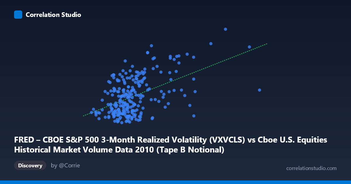
FRED – CBOE S&P 500 3-Month Realized Volatility (VXVCLS) vs Cboe U.S. Equities Historical Market Volume Data 2010 (Tape B Notional)
- Pearson correlation (r)
- 0.4991
- Spearman correlation
- 0.399
- p-value
- 0
- Sample size (n)
- 252
- 95% confidence interval
- 0.4002 to 0.5865
- Granger causality
- Y → X
- Granger optimal lag
- 1
AI analysis
Analysis: CBOE S&P 500 3-Month Realized Volatility vs. Tape B Notional Volume (2010)
Relationship Overview
The scatterplot reveals a moderate positive relationship between CBOE S&P 500 3-Month Realized Volatility (VXVCLS) and Tape B Notional trading volume across U.S. equity exchanges in 2010. As volatility rises, notional volume traded on Tape B venues tends to increase — a directionally intuitive finding, since periods of heightened uncertainty typically drive elevated trading activity. The linear regression equation (y = 1.09×10⁻⁹x + 19.22) confirms this upward slope, though the intercept near 19.22% volatility suggests a meaningful baseline level of implied volatility even at very low volume regimes. The relationship is real but far from deterministic, as substantial scatter around the regression line is immediately apparent throughout the distribution.
Correlation Strength and Statistical Significance
The Pearson correlation of r = 0.499 indicates a moderate positive association, but the more policy-relevant figure is R² = 0.249 — meaning that Tape B notional volume explains only about 25% of the variance in 3-month realized volatility. Three-quarters of volatility's variation is driven by factors entirely outside this model. The 95% confidence interval for r of [0.40, 0.59] is reasonably tight given n = 252, and the p-value of effectively zero (against N = 3,302) confirms this is not a chance artifact. Crucially, the Granger causality results break the symmetry: Y→X is statistically significant (F = 7.66, p = 0.006), while X→Y falls short of significance (F = 3.32, p = 0.070). This means volatility (Y) temporally predicts subsequent notional volume (X) with a 1-period lag — not the reverse — suggesting traders respond to volatility signals rather than volume driving volatility. This is a meaningful directional finding for market microstructure interpretation.
Patterns, Clusters, and Outliers
Several structural features stand out in the point cloud. The bulk of observations cluster in the lower-left region — roughly X < 6×10⁹ and Y between 19–28 — representing the more quiescent, range-bound trading environment that characterized much of early-to-mid 2010. A distinct upper-right cluster is visible at very high notional volumes (X 8–15×10⁹), consistently associated with elevated volatility readings above 30%, likely corresponding to the May 2010 Flash Crash and European sovereign debt stress periods. The extreme outlier near X ≈ 15.1×10⁹ with Y ≈ 36.6% stands out sharply and almost certainly reflects the Flash Crash on May 6, 2010. There is also a suggestion of heteroscedasticity — variance in Y appears to fan outward as X increases — which may slightly undermine the linear model's assumptions and inflate uncertainty at high-volume extremes.
Confounding Factors and Caveats
Several important caveats apply. First, the axes appear to be swapped relative to intuitive convention: VXVCLS (volatility) is on the X-axis and notional volume on Y, yet Granger causality runs Y→X, meaning the "effect" variable is plotted as the predictor — a presentation that could mislead casual readers. Second, both variables are jointly driven by macroeconomic shocks (e.g., the Flash Crash, Greek debt crisis), meaning much of the observed correlation may reflect common external causation rather than a direct structural link. Third, Tape B specifically represents a subset of venues (NYSE American, regional exchanges), and its notional volume dynamics may differ from aggregate market behavior, limiting generalizability. Finally, 2010 is a single calendar year with idiosyncratic events, and the relationship may not hold across different volatility regimes or market structures.
Actionable Insights and Further Investigation
The Granger causality finding — that volatility leads volume with a 1-day lag — has practical implications for intraday and short-term trading strategy: elevated VXVCLS readings could serve as a leading signal for anticipating heightened Tape B activity the following session, useful for liquidity management, execution timing, or market-making positioning. However, given that only 25% of variance is explained, this signal should be combined with other predictors. Further investigation should include: (1) extending the time series beyond 2010 to test whether the Granger relationship is stable across regimes; (2) non-linear modeling (e.g., quantile regression or spline fits) to better capture the apparent heteroscedasticity at high volumes; (3) controlling for VIX term structure and macro event dummies to isolate the structural volume-volatility channel; and (4) comparing Tape B behavior against Tape A and C venues to determine whether this relationship is venue-specific or market-wide.
X dataset: Cboe U.S. Equities Historical Market Volume Data 2010
Y dataset: FRED – CBOE S&P 500 3-Month Realized Volatility
Part of experiment: Daily - Cboe U.S. Equities Historical Market Volume Data 2010 vs FRED – CBOE S&P 500 3-Month Realized Volatility