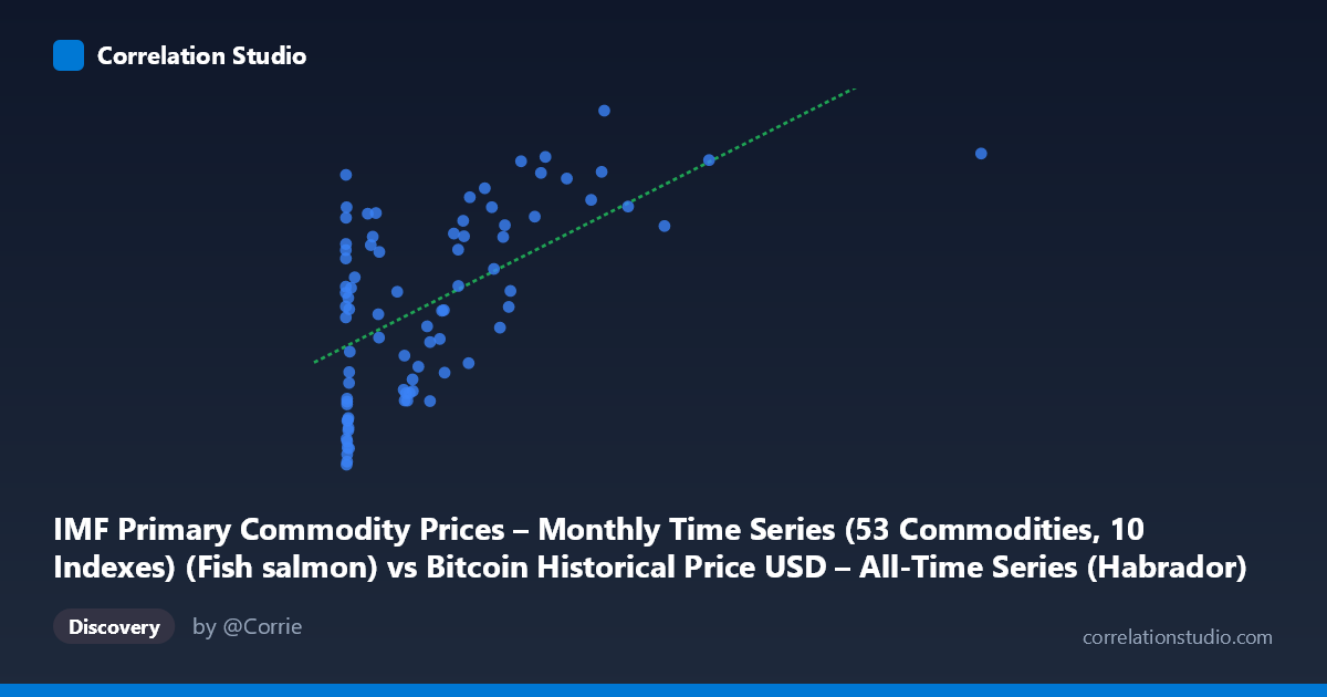
IMF Primary Commodity Prices – Monthly Time Series (53 Commodities, 10 Indexes) (Fish salmon) vs Bitcoin Historical Price USD – All-Time Series (Habrador) (Price)
- Pearson correlation (r)
- 0.5838
- Spearman correlation
- 0.5206
- p-value
- 0
- Sample size (n)
- 83
- 95% confidence interval
- 0.4211 to 0.7101
- Granger causality
- None
- Granger optimal lag
- 1
- Time coverage
- 2010-08-01 to 2017-06-01
AI analysis
Analysis: Bitcoin Price vs. Fish Salmon Commodity Index
1. Relationship Overview
The scatterplot shows a moderate positive association between the fish salmon commodity price index (X) and Bitcoin's historical price (Y). The relationship appears non-linear on visual inspection: at low X values (roughly 0–50), Y spans an enormous range (4.2 to 7.8), producing a dense vertical scatter near the origin. As X increases beyond ~200, the points thin out and trend upward more consistently, suggesting the relationship may be better characterized as logarithmic or exhibiting heteroscedasticity rather than strictly linear.
2. Strength, Direction, and Statistical Confidence
The correlation coefficient (r = 0.584) indicates a moderate positive relationship, with r² = 0.341 meaning only about 34% of the variance in Y is explained by X — leaving roughly two-thirds of Bitcoin's price variation unaccounted for by this commodity index alone. The 95% CI [0.421, 0.710] is reasonably tight and excludes zero, and the extremely small p-value (6.9×10⁻⁹) confirms this correlation is statistically robust and not due to chance in this sample. However, statistical significance should not be conflated with practical predictive power given the modest r².
Critically, the Granger causality tests show no significant predictive direction in either direction (X→Y: p=0.877; Y→X: p=0.107). This strongly suggests the correlation is not causal in a temporal/dynamic sense — neither series helps forecast the other's future values based on past values. This is a key finding: despite the positive contemporaneous correlation, this is likely a spurious or confounded relationship rather than one variable driving the other.
3. Notable Patterns and Outliers
The data shows a clear clustering pattern: a dense cloud of low-X points (X < 50) with highly variable Y (4.2–7.8), and a sparser set of high-X points (X 600) that consistently show higher Y values (7–8.6). This creates an impression of correlation that may be driven more by the temporal ordering of the two time series (both trending upward over 2010–2017) than by any genuine economic linkage. A few high-leverage points (X ≈ 1402, 2452) sit far from the bulk of the data and may disproportionately influence the linear fit. The near-vertical scatter at very low X values (X < 1) with Y ranging from 6.0 to 7.9 is particularly striking and inconsistent with a clean linear model.
4. Confounding Factors and Caveats
This is almost certainly a spurious correlation driven by shared time trends. Bitcoin price experienced dramatic secular growth from 2010–2017, and if the salmon/commodity index also trended upward (even for unrelated macroeconomic reasons — inflation, general commodity bull markets, currency effects), the two series will correlate simply because both are increasing over time, not because of any causal or economic link between salmon prices and cryptocurrency. The lack of Granger causality reinforces this: there's no lead-lag predictive structure, only co-movement in levels. Additionally, both series are highly non-stationary (especially Bitcoin, which grew by orders of magnitude), violating assumptions of standard Pearson correlation and OLS regression, which can inflate apparent correlation between trending non-stationary series.
5. Recommendations for Further Investigation
Given the near-certainty of a spurious time-trend relationship, analysts should: (1) detrend or difference both series (e.g., use month-over-month % changes) and re-run the correlation — this typically eliminates spurious trend-driven correlations; (2) test for cointegration rather than relying on simple correlation, since both series may share a stochastic trend; (3) treat this pairing as a cautionary example of "nonsense regression" in time series analysis rather than a meaningful economic relationship. Practically, this correlation should not be used for trading, forecasting, or hedging decisions — the absence of Granger causality is the most important finding here, overriding the seemingly significant r and p-value.
X dataset: Bitcoin Historical Price USD – All-Time Series (Habrador)
Y dataset: IMF Primary Commodity Prices – Monthly Time Series (53 Commodities, 10 Indexes)
Part of experiment: Bitcoin - Bitcoin Historical Price USD – All-Time Series (Habrador) vs IMF Primary Commodity Prices – Monthly Time Series (53 Commodities, 10 Indexes)