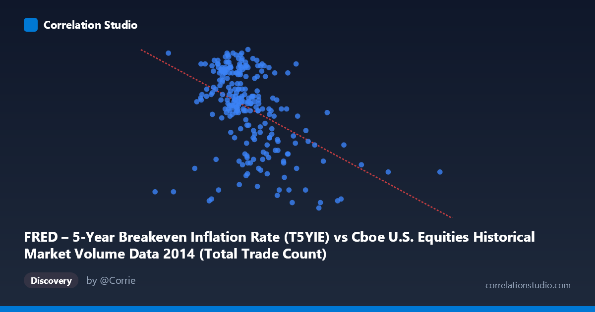
FRED – 5-Year Breakeven Inflation Rate (T5YIE) vs Cboe U.S. Equities Historical Market Volume Data 2014 (Total Trade Count)
- Pearson correlation (r)
- -0.4466
- Spearman correlation
- -0.453
- p-value
- 0
- Sample size (n)
- 250
- 95% confidence interval
- -0.5407 to -0.3415
- Granger causality
- None
- Granger optimal lag
- 1
AI analysis
Analysis: 5-Year Breakeven Inflation Rate vs. U.S. Equities Total Trade Count (2014)
Relationship Overview The scatterplot reveals a moderate negative relationship between U.S. equity market trade counts (X-axis) and the 5-year breakeven inflation rate (Y-axis) across 2014. As daily trade volume increases, inflation expectations tend to be lower, and conversely, periods of lower trading activity are associated with higher breakeven inflation readings. The linear regression equation (y = -2.46×10⁻⁷x + 2.233) quantifies this inverse slope, with trade counts ranging widely from roughly 920,000 to over 4.4 million while inflation expectations cluster between approximately 1.17% and 2.05%. The cloud of points shows considerable scatter around the regression line, suggesting the relationship, while real, is far from deterministic.
Correlation Strength and Statistical Significance The Pearson correlation of r = -0.447 indicates a moderate negative association. However, the coefficient of determination r² = 0.1995 means that only ~20% of the variance in the 5-year breakeven inflation rate is explained by trade count — leaving roughly 80% of the variation attributable to other factors. The 95% confidence interval of [-0.54, -0.34] is entirely negative, confirming directional consistency, and the p-value of 1.17×10⁻¹³ is highly statistically significant given n=250, ruling out chance as an explanation. That said, statistical significance here is partly a function of the large underlying population (N=3,686), so practical significance deserves independent scrutiny. Critically, Granger causality tests find no significant predictive direction in either direction (X→Y: F=0.39, p=0.54; Y→X: F=0.07, p=0.80), meaning neither variable temporally predicts the other at the tested lag — the correlation reflects co-movement, not a leading/lagging predictive signal.
Patterns, Clusters, and Outliers The data exhibit a broad, diffuse central cluster concentrated between approximately 1.6M–2.5M trade counts and 1.6–2.05% inflation expectations, where the negative trend is most visible. Several notable features emerge: - High inflation / low volume observations (upper-left quadrant, ~1.0–1.5M trades, ~1.9–2.05%) suggest early-year or low-volatility periods when inflation expectations were elevated and markets were quieter - Low inflation / high volume points (lower-right, 3.0M trades, ~1.2–1.4%) likely correspond to market stress or high-activity periods (e.g., late 2014 oil price-driven inflation expectations collapse) coinciding with elevated trading - The single extreme outlier at ~4.4M trade count (rightmost point) warrants investigation as a potential data anomaly or an exceptionally high-volume trading day - A few anomalous low-inflation points (~1.2%) at moderate trade counts (~1.1–1.6M) break the general trend and suggest non-linearity at the tails
Confounding Factors and Caveats Several important caveats apply. First, temporal confounding is the primary concern: both series evolve through time in 2014, and shared time trends (e.g., the dramatic oil price decline in H2 2014 simultaneously suppressed inflation expectations and may have altered trading patterns) could be driving the apparent correlation spuriously. Second, the axis labels appear inverted in the metadata — the X-axis column name references "FRED – 5-Year Breakeven Inflation Rate" while the Y-axis references "Total Trade Count," suggesting a possible dataset assignment inconsistency that should be verified before drawing conclusions. Third, market microstructure changes, regulatory shifts, and seasonal trading patterns in 2014 could independently influence trade counts without any causal link to inflation. Finally, the 20% explained variance ceiling implies that macroeconomic factors (Fed policy expectations, geopolitical risk, equity volatility regimes) likely dominate both series independently.
Actionable Insights and Further Investigation Despite the lack of Granger causality, the co-movement warrants deeper exploration. Recommended next steps include: (1) Decomposing the time series to remove shared trends before re-computing correlations, isolating whether the relationship persists in residuals; (2) Segmenting by market regime — specifically separating pre- and post-October 2014 (when oil prices collapsed) to test whether the correlation is regime-dependent; (3) Testing additional lags beyond the single period examined in Granger tests, as inflation expectations may respond to sustained volume patterns rather than single-day shifts; (4) Including VIX or equity volatility as a control variable, since volatility plausibly drives both trade counts and risk-adjusted inflation expectations simultaneously; and (5) Verifying the axis/dataset assignment to ensure the correlation direction is being interpreted correctly given the metadata inconsistency noted above.
X dataset: Cboe U.S. Equities Historical Market Volume Data 2014
Y dataset: FRED – 5-Year Breakeven Inflation Rate
Part of experiment: Daily - Cboe U.S. Equities Historical Market Volume Data 2014 vs FRED – 5-Year Breakeven Inflation Rate