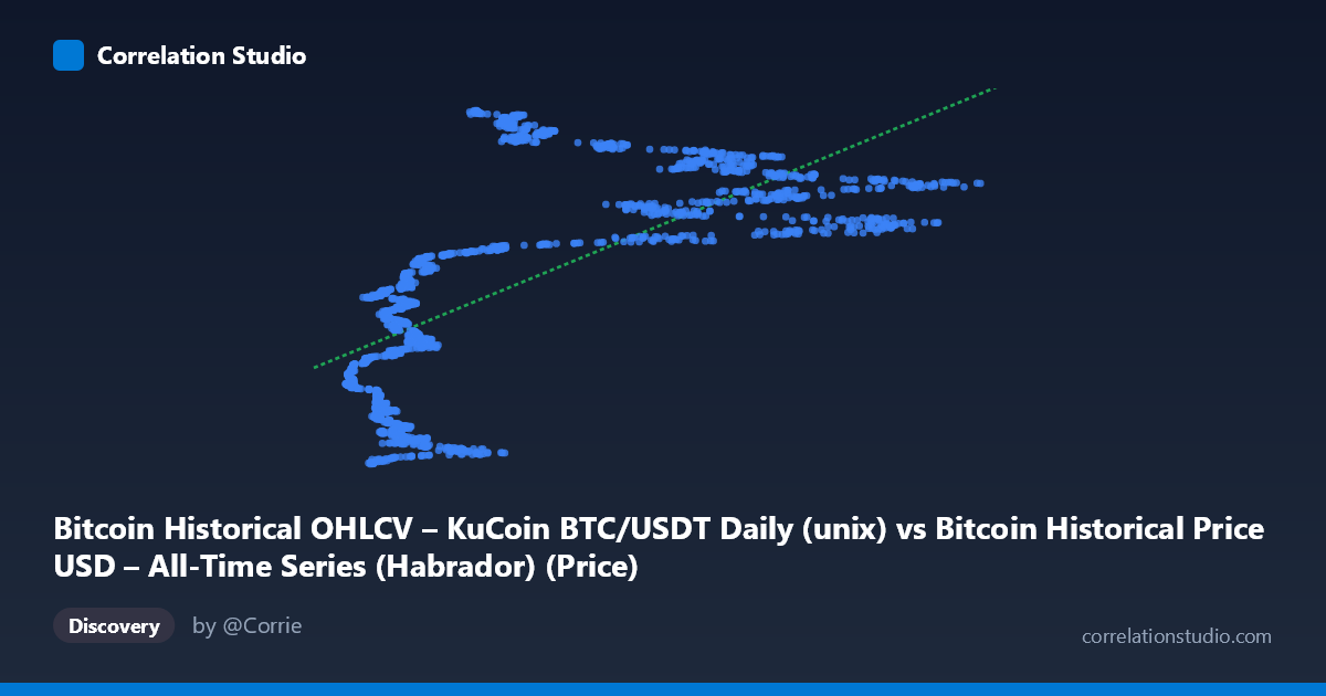
Bitcoin Historical OHLCV – KuCoin BTC/USDT Daily (unix) vs Bitcoin Historical Price USD – All-Time Series (Habrador) (Price)
- Pearson correlation (r)
- 0.6738
- Spearman correlation
- 0.7541
- p-value
- 0
- Sample size (n)
- 1861
- 95% confidence interval
- 0.6482 to 0.6979
- Granger causality
- None
- Granger optimal lag
- 10
- Time coverage
- 2017-10-19 to 2022-11-29
- Recomputed on refreshed data
- 2026-10-24 (r was 0.6738)
AI analysis
Analysis of Bitcoin Price vs. Time Relationship
1. What the Visualization Reveals
This scatterplot is essentially plotting Bitcoin's historical price (X-axis, in USD) against the Unix timestamp of when that price occurred (Y-axis). This is an unconventional pairing — rather than showing two independent market variables, it's showing price against its own occurrence date. The result reveals how BTC price levels are distributed across the ~5-year window from October 2017 to November 2022, capturing multiple bull/bear cycles (the 2017-18 peak and crash, the 2020-21 bull run, and the 2022 bear market).
2. Strength, Direction, and Statistical Confidence
The correlation is moderate-to-strong and positive (r = 0.674), with an R² of 0.454 indicating that only 45.4% of the variance in the timestamp variable is explained by price (or vice versa) in a linear sense — meaning more than half the variance is driven by other structure (likely non-linear cyclical patterns rather than a simple linear trend). The 95% CI [0.648, 0.698] is tight, and the p-value of ~0 confirms this relationship is highly statistically significant and not due to chance, which is expected given the large sample (n=1,861) and the fact that price data is inherently non-independent (autocorrelated) over time.
Critically, the Granger causality test shows no significant predictive direction in either direction (X→Y: p=0.865; Y→X: p=0.088, only marginally approaching significance). This makes sense structurally: X (price) and Y (timestamp) can't "Granger-cause" each other in a meaningful economic sense — time flows forward deterministically and doesn't respond to price, and price at lag structures here doesn't cleanly forecast time. This result underscores that the linear correlation here reflects a within-sample trend association, not a predictive causal relationship.
3. Notable Patterns and Non-linear Features
The sample points reveal a clearly non-linear, cyclical structure disguised by the linear correlation statistic: - Low X values (~$3,600–$10,000) map to two distinct time clusters: late 2017/early 2018 (pre-bull-run) AND mid-late 2020/2022 crash periods — showing price returning to similar low levels at very different times. - High X values (~$40,000–$60,000) cluster tightly in 2021–2022, reflecting the bull run peak and subsequent elevated trading range. - The relationship is better described as cyclical/oscillating (boom-bust-boom) rather than monotonic, meaning a single linear regression line (y = 1848.21x + 1.55×10⁹) poorly captures the true dynamics — it averages over multiple distinct regimes.
4. Confounding Factors and Caveats
The core caveat is that this is a reflexive relationship: X (price) is drawn from the same historical series as Y (timestamp), so correlating "price" with "time of price" is fundamentally different from correlating two independent economic variables. Apparent linear correlation is an artifact of Bitcoin's overall upward price trajectory over the sampled years, not evidence of any causal or predictive mechanism. Additionally, financial time series exhibit strong autocorrelation and regime-switching behavior (bull/bear cycles), violating the i.i.d. assumptions behind standard correlation/regression inference — the true "effective sample size" is much smaller than n=1,861 suggests.
5. Actionable Insights
- Avoid over-interpreting r²=0.45 as meaningful predictive power — given the reflexive X/Y setup and lack of Granger causality, this correlation should not be used for forecasting. - Segment the data by market regime (2017-18 cycle, 2020-21 bull run, 2022 bear market) and analyze each separately, or apply time-series-appropriate models (e.g., ARIMA, regime-switching models) rather than linear regression. - Verify the data pairing intent — if the goal was to study relationship between BTC price and another asset/indicator, confirm the correct variables are mapped to X and Y, as the current setup (price vs. its own timestamp) limits the analytical value of correlation/Granger statistics.
X dataset: Bitcoin Historical Price USD – All-Time Series (Habrador)
Y dataset: Bitcoin Historical OHLCV – KuCoin BTC/USDT Daily
Part of experiment: Bitcoin - Bitcoin Historical Price USD – All-Time Series (Habrador) vs Bitcoin Historical OHLCV – KuCoin BTC/USDT Daily