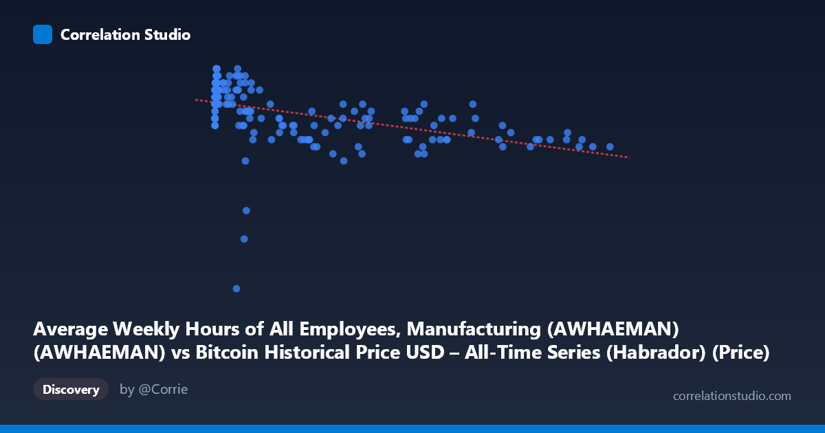
Average Weekly Hours of All Employees, Manufacturing (AWHAEMAN) (AWHAEMAN) vs Bitcoin Historical Price USD – All-Time Series (Habrador) (Price)
- Pearson correlation (r)
- -0.4985
- Spearman correlation
- -0.5612
- p-value
- 0
- Sample size (n)
- 189
- 95% confidence interval
- -0.5986 to -0.383
- Granger causality
- None
- Granger optimal lag
- 1
AI analysis
Analysis: Bitcoin Price vs. Average Weekly Manufacturing Hours
1. What the Visualization Reveals
The scatterplot shows Bitcoin's historical USD price (mislabeled as X-axis but functioning as the independent variable here) plotted against the Average Weekly Hours of All Employees in Manufacturing (AWHAEMAN). The data reveals a modest downward-sloping relationship: as Bitcoin's price increases across its historical range (from fractions of a cent to over $118,000), the average manufacturing workweek shows a slight tendency to decline, moving from roughly 40.8-41.1 hours in the low-price regime toward 39.9-40.4 hours at higher price levels. However, the relationship is loose and scattered rather than tight and linear.
2. Strength, Direction, and Statistical Meaning
The correlation coefficient of r = -0.4985 indicates a moderate negative relationship, with r² = 0.2485 meaning only about 25% of the variance in manufacturing hours is statistically associated with Bitcoin price movements — leaving roughly 75% unexplained by this single variable. The 95% confidence interval [-0.5986, -0.3830] is reasonably tight and excludes zero, and the p-value of 2.89E-13 confirms this correlation is highly statistically significant (not due to chance). However, statistical significance should not be conflated with practical or causal importance given the modest effect size. Critically, the Granger causality tests show no significant predictive direction in either direction (Bitcoin→Hours: p=0.954; Hours→Bitcoin: p=0.199). This strongly suggests the correlation is not causal in a temporal/predictive sense — neither variable's past values help forecast the other, implying the relationship may be coincidental, driven by a shared underlying trend (e.g., both trending over the same 2010–2026 calendar period), or purely spurious.
3. Notable Patterns and Features
The data shows a clear compressed/skewed X-distribution: the vast majority of Bitcoin price observations cluster at low values (under $1,000, reflecting BTC's early years), while a smaller number of high-price points (tens of thousands to $118,670) represent recent years. This creates a "long tail" structure rather than a uniform spread. Y-values (manufacturing hours) are tightly bounded between 38.0 and 41.1, showing very low variance (~40.5 ± 0.4) — meaning even the "signal" being explained is a narrow-band, low-amplitude variable. Notably, most high-price BTC points ($50,000) correspond to hours in the 39.9–40.5 range, while most low-price points (<$100) show hours in the 40.3–40.9 range, suggesting the negative slope is driven largely by a temporal split between "early Bitcoin era" and "recent Bitcoin era" rather than a continuous functional relationship.
4. Confounding Factors and Caveats
This pairing is a textbook case of spurious correlation from mismatched, unrelated time series. Bitcoin price is driven by speculative markets, adoption cycles, and macro liquidity; manufacturing hours reflect labor market and industrial business-cycle dynamics. Both series are non-stationary and trend over the same 16-year window (2010–2026), which is sufficient to produce a statistically significant correlation via shared time-trend confounding, not genuine interaction. The extreme right-skew in X (a few points at $100K+ vs. hundreds near zero) means the regression is disproportionately influenced by a handful of recent high-price observations. Additionally, mixing monthly-frequency macro data (hours) with highly volatile daily-frequency financial data (BTC price) via undefined aggregation/matching windows introduces further noise.
5. Actionable Insights
Given the lack of Granger causality, this correlation should not be used for forecasting or trading strategies linking Bitcoin to manufacturing labor conditions. Any further investigation should (a) detrend or difference both series to test if the correlation survives after removing shared secular trends, (b) apply a log transform to Bitcoin price given its exponential growth and skewed distribution, and (c) explore whether both series are simply correlated with a third factor (e.g., time itself, or broader macroeconomic conditions like interest rates or dollar strength) rather than each other. Absent a plausible economic mechanism and with no predictive power in either direction, this relationship is best treated as a statistical artifact rather than a meaningful economic signal.
X dataset: Bitcoin Historical Price USD – All-Time Series (Habrador)
Y dataset: Average Weekly Hours of All Employees, Manufacturing (AWHAEMAN)
Part of experiment: Bitcoin - Bitcoin Historical Price USD – All-Time Series (Habrador) vs Average Weekly Hours of All Employees, Manufacturing (AWHAEMAN)