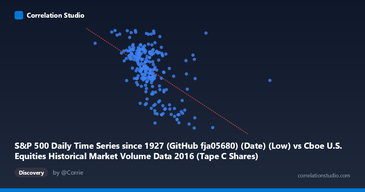
S&P 500 Daily Time Series since 1927 (GitHub fja05680) (Date) (Low) vs Cboe U.S. Equities Historical Market Volume Data 2016 (Tape C Shares)
- Pearson correlation (r)
- -0.522
- Spearman correlation
- -0.52
- p-value
- 0
- Sample size (n)
- 252
- 95% confidence interval
- -0.6065 to -0.4259
- Granger causality
- None
- Granger optimal lag
- 4
AI analysis
Analysis: S&P 500 Low Price vs. Cboe Tape C Share Volume (2016)
Relationship Overview The scatterplot reveals a negative relationship between the S&P 500 daily low price (X-axis) and Cboe Tape C share volume (Y-axis) across 252 trading days in 2016. As the S&P 500 index reached higher price levels, Tape C share volume tended to decline, and conversely, lower index price levels were associated with elevated trading volume. This inverse pattern is consistent with a well-known market dynamic: periods of market stress or decline typically generate heightened trading activity as investors rebalance, hedge, or liquidate positions, while calmer, rising markets tend to see more subdued volume. The linear regression equation (y = −2.02×10⁻⁶x + 2352.43) quantifies this negative slope, showing that each unit increase in the S&P 500 low is associated with a small but consistent decrease in share volume.
Correlation Strength and Statistical Significance The Pearson correlation of r = −0.522 indicates a moderate negative association. However, the coefficient of determination (r² = 0.2725) tempers this interpretation considerably — only 27.3% of the variance in Tape C share volume is explained by the S&P 500 low price level, leaving roughly 73% of variability attributable to other factors. The 95% confidence interval of [−0.607, −0.426] is entirely negative and reasonably tight, confirming directional reliability, and the p-value of effectively zero (derived from a population N of 3,622) confirms this relationship is highly unlikely to be due to chance. That said, statistical significance here is partly a function of sample size, and practical significance should be evaluated carefully given the modest r². Critically, the Granger causality tests returned no significant result in either direction (X→Y: F = 0.98, p = 0.42; Y→X: F = 1.47, p = 0.21), meaning that neither variable meaningfully predicts the other's future values at the optimal four-period lag. This rules out a straightforward temporal predictive relationship and suggests any link is contemporaneous rather than leading/lagging.
Notable Patterns, Clusters, and Outliers The scatterplot exhibits a broad, somewhat diffuse cloud rather than a tight linear band, reflecting the modest r² value. Several noteworthy features stand out. A cluster of high-volume, lower-price observations appears at the left side of the chart (S&P 500 lows in the ~95M–120M range, Tape C shares above 2,150–2,265), likely corresponding to the volatile early 2016 period (January–February) when equity markets sold off sharply. Conversely, a cluster of lower-volume, higher-price points at the right side (~150M–175M range) likely reflects the calmer mid-to-late 2016 rally. A few apparent outliers are visible — most notably a point near (99.8M, 2265) representing an exceptionally high Tape C volume day, and several low-volume, low-price days around (166M–175M, 1848–1874) that suggest isolated calm trading sessions during market weakness. These outliers could meaningfully influence the regression slope and warrant individual investigation.
Confounding Factors and Caveats Several important caveats apply. First, the axes appear to be mislabeled or counterintuitively assigned — the X-axis values (~51M to 315M) are described as S&P 500 "Low" prices, but the S&P 500 traded in the 1,800–2,270 range in 2016, suggesting these X values may actually represent Cboe market volume metrics, and Y values (~1,810–2,266) align more naturally with S&P 500 price levels. This potential label swap would invert the causal framing entirely and should be verified before drawing any conclusions. Second, seasonality and calendar effects (e.g., holiday-shortened weeks, quarterly expiration events) independently affect both volume and market behavior. Third, macroeconomic events in 2016 — the Brexit vote, U.S. presidential election, and Federal Reserve rate decisions — created discrete volatility episodes that could drive both variables simultaneously, inflating correlation through shared external shocks rather than a direct relationship. Fourth, Tape C specifically covers NYSE Arca-listed securities, making this a partial market snapshot rather than a comprehensive volume measure.
Actionable Insights and Further Investigation Practitioners should not rely on S&P 500 price levels alone to forecast Tape C volume, given the absence of Granger causality and the limited explained variance. More productive next steps would include: (1) incorporating volatility measures (e.g., VIX) as covariates, since fear and volatility likely mediate the price–volume relationship more directly; (2) segmenting the data by market regime (trending vs. mean-reverting periods) to test whether the negative correlation holds uniformly or is driven primarily by stress episodes; (3) resolving the axis labeling ambiguity to ensure the directionality of findings is correctly interpreted; and (4) extending the analysis across multiple years to assess whether this 2016-specific pattern generalizes, since 2016 contained unusual political and macro events. A multivariate regression incorporating lagged VIX, trading day-of-week, and options expiration indicators would likely substantially improve explanatory power beyond the current 27%.
X dataset: Cboe U.S. Equities Historical Market Volume Data 2016
Y dataset: S&P 500 Daily Time Series since 1927 (GitHub fja05680) (Date)
Part of experiment: Daily - Cboe U.S. Equities Historical Market Volume Data 2016 vs S&P 500 Daily Time Series since 1927 (GitHub fja05680) (Date)