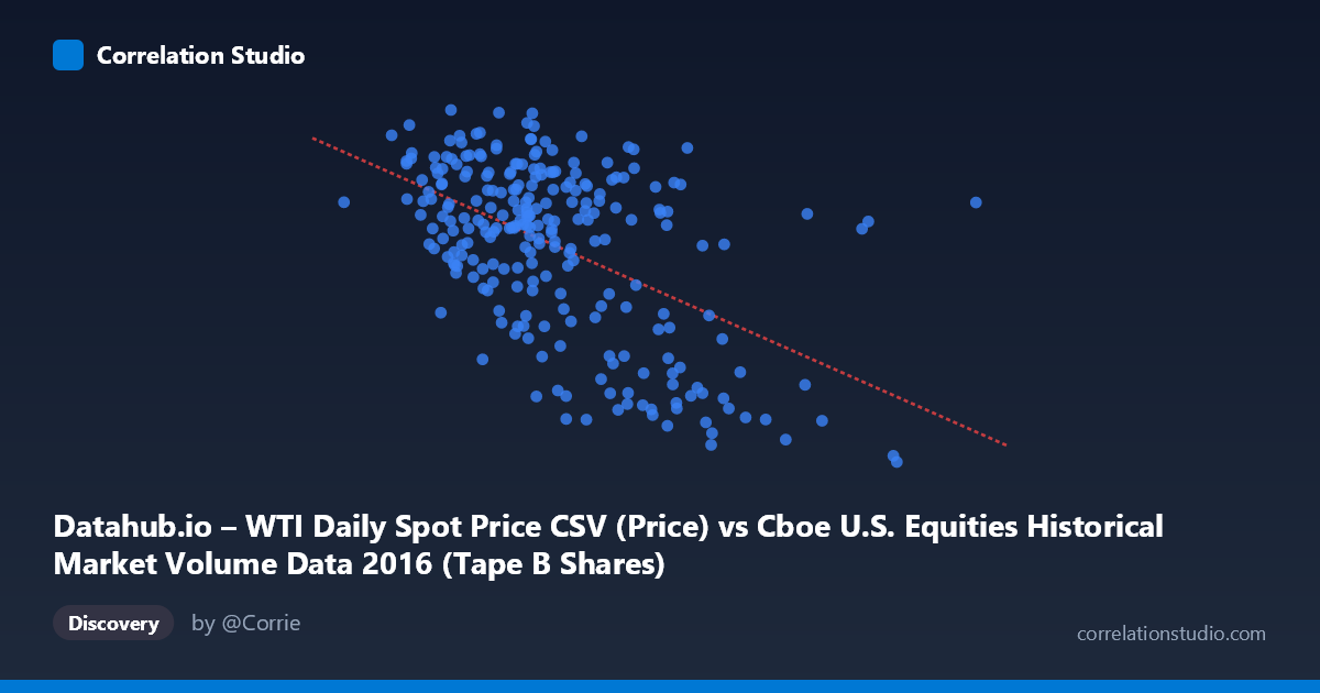
Datahub.io – WTI Daily Spot Price CSV (Price) vs Cboe U.S. Equities Historical Market Volume Data 2016 (Tape B Shares)
- Pearson correlation (r)
- -0.5218
- Spearman correlation
- -0.4332
- p-value
- 0
- Sample size (n)
- 252
- 95% confidence interval
- -0.6062 to -0.4256
- Granger causality
- None
- Granger optimal lag
- 1
AI analysis
Analysis: WTI Oil Price vs. Cboe Tape B Share Volume (2016)
Relationship Overview The scatterplot reveals a moderate negative relationship between U.S. equity market volume (specifically Tape B shares, representing NYSE American-listed securities) and the WTI daily spot price of crude oil. As oil prices rise, Tape B share volume tends to decline, and conversely, periods of lower oil prices coincide with higher trading volumes. The linear regression equation (y = -1.16169E⁻⁰⁷x + 55.74) confirms this inverse slope, though the scatter around the regression line is substantial, indicating considerable unexplained variance in the relationship.
Correlation Strength and Statistical Framing The Pearson correlation of r = -0.5218 indicates a moderate negative association, but the explanatory power is notably limited: r² = 0.2722 means only 27.2% of the variance in Tape B share volume is explained by WTI price movements, leaving nearly three-quarters of the variation attributable to other factors. The 95% confidence interval [-0.6062, -0.4256] is reasonably tight and does not cross zero, lending credibility to the negative direction. With a p-value effectively at zero and N = 3,622, the correlation is highly statistically significant and unlikely to be a sampling artifact. However, the Granger causality results are telling — neither direction (X→Y: F = 1.02, p = 0.31; Y→X: F = 1.43, p = 0.23) achieves significance, meaning neither variable temporally predicts the other at a one-period lag. Statistical correlation exists, but there is no evidence of directional temporal causation between oil prices and Tape B volume within this dataset's time structure.
Patterns, Clusters, and Outliers Several notable structural features emerge from the sampled points. There is a visible cluster of high-volume trading days (Tape B shares ~45–52) concentrated in the lower oil price range (~$75M–$105M notional, roughly corresponding to lower WTI values), suggesting that equity market activity in this segment was elevated when oil was cheaper in early-to-mid 2016. A distinct cluster of low-volume, high-price outliers is apparent — points such as (170,560,180, 29.55) and (133,797,318, 33.21) suggest specific high-oil-price days where Tape B volume dropped sharply, potentially corresponding to late 2016 as oil recovered post-OPEC agreement. The point at (78,935,242, 51.44) stands out as an unusually high volume day at relatively low oil prices. The overall pattern is not cleanly linear — there appears to be a plateau of moderate volume across a wide mid-range of oil prices, with volume degradation becoming more pronounced only at the higher oil price extremes.
Confounding Factors and Caveats Several important caveats temper straightforward interpretation. First, 2016 was a structurally unusual year for both markets: oil prices began near multi-year lows (~$26–$30/barrel in January–February) and recovered significantly through the year following the OPEC production agreement in late November, meaning time itself is a strong lurking variable driving both series simultaneously. Second, Tape B volume is a narrow slice of U.S. equity market activity (NYSE American-listed stocks), and many of these are energy-sector companies, which could create a mechanical link rather than a broad macroeconomic one. Third, broader market volatility events (e.g., Brexit in June 2016, the U.S. election in November) likely spiked or suppressed equity volumes independently of oil prices, creating confounded data points. The absence of Granger causality further underscores that this correlation may be largely spurious co-movement driven by shared macroeconomic conditions rather than any direct functional relationship.
Actionable Insights and Further Investigation Given these findings, analysts should avoid treating this correlation as a reliable trading signal or causal mechanism without deeper investigation. Recommended next steps include: (1) controlling for time trend by detrending both series to isolate whether the correlation persists beyond the shared directional drift of 2016; (2) segmenting by market regime — testing whether the correlation holds separately in Q1 (low oil, high volatility) versus Q4 (recovering oil, post-election volume surge); (3) examining sector composition of Tape B listings to determine what fraction are energy-related, which would explain mechanical co-movement; and (4) testing longer time horizons across multiple years to assess whether this 2016 relationship is structural or episodic. Incorporating volatility indices (VIX) and broader macro controls (USD index, equity sector flows) into a multivariate model would likely substantially improve explanatory power beyond the modest 27.2% currently captured.
X dataset: Cboe U.S. Equities Historical Market Volume Data 2016
Y dataset: Datahub.io – WTI Daily Spot Price CSV
Part of experiment: Daily - Cboe U.S. Equities Historical Market Volume Data 2016 vs Datahub.io – WTI Daily Spot Price CSV