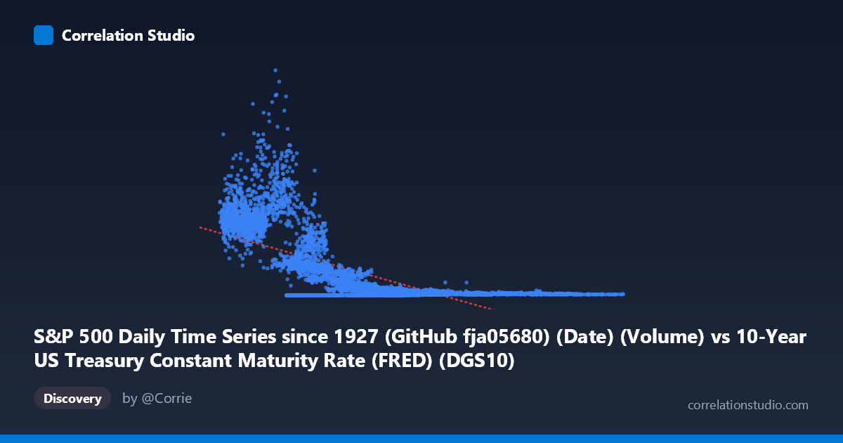
S&P 500 Daily Time Series since 1927 (GitHub fja05680) (Date) (Volume) vs 10-Year US Treasury Constant Maturity Rate (FRED) (DGS10)
- Pearson correlation (r)
- -0.6535
- Spearman correlation
- -0.5365
- p-value
- 0
- Sample size (n)
- 14441
- 95% confidence interval
- -0.6627 to -0.644
- Granger causality
- None
- Granger optimal lag
- 10
AI analysis
Analysis: S&P 500 Trading Volume vs. 10-Year Treasury Yield
1. Relationship Overview
The scatterplot reveals a negative relationship between S&P 500 daily trading volume (X) and the 10-year US Treasury constant maturity yield (Y), spanning nearly six decades of daily financial data (1962–2019). The linear regression equation (y = -3.76×10⁸x + 3.49×10⁹) indicates that as trading volume increases, Treasury yields tend to decrease. This inverse pattern is visually apparent in the sample points: very high yields (e.g., 8.56B at x≈3.18, 9.12B at x≈3.29) cluster at low volume values, while higher volume observations (x 8–10) are associated with much lower yields. This temporal dynamic makes intuitive sense — modern markets have vastly higher trading volumes than early decades, while the high-yield era of the 1970s–80s has given way to the low-yield environment of the 2000s–2010s.
2. Correlation Strength, Direction, and Causality
The Pearson correlation of r = -0.6535 reflects a moderate-to-strong negative association, and with r² = 0.4270, trading volume accounts for approximately 42.7% of the variance in Treasury yields — a substantial but far from complete explanation. The 95% confidence interval of [-0.6627, -0.6440] is exceptionally narrow, and the p-value of effectively zero (across N = 16,799 observations) confirms this relationship is highly statistically significant and not attributable to sampling error. However, the Granger causality results are unambiguous in their null finding: neither direction (X→Y nor Y→X) achieves significance at any meaningful level (F = 0.48, p = 0.90 for volume predicting yield; F = 0.53, p = 0.87 for yield predicting volume, both at optimal lag 10). This means that despite the strong correlation, neither variable temporally predicts the other — the relationship is associative, not directionally causal in a time-series sense.
3. Notable Patterns, Clusters, and Outliers
The sample points reveal two visually distinct clusters that dominate the scatterplot's structure. A dense cluster of low-volume, high-yield observations (x < 5, y 1–9B) corresponds to the pre-digitization, high-interest-rate era of the 1960s–80s. A second cluster of moderate-to-high volume, low-yield observations (x 6, y < 500M) reflects the post-2000 landscape of electronic trading and quantitative easing. Several apparent outliers exist — notably points like (3.87, 3.28M) at very low volume and low yield, and (8.96, 40.74M) at moderate volume — suggesting the relationship is not uniformly distributed. The extreme Y-axis range (1.95M to 10.62B) and right-skewed volume distribution imply that a log-transformation of Y would likely reveal more linear and interpretable structure than the current linear fit captures.
4. Confounding Factors and Caveats
The most critical caveat is that both variables are jointly driven by time itself — this correlation almost certainly reflects two independent secular trends rather than any direct financial mechanism. Trading volume has risen dramatically due to technological change, market democratization, algorithmic trading, and index fund growth. Treasury yields, meanwhile, followed the Volcker-era peak in the early 1980s and a subsequent 35-year secular decline driven by disinflation, monetary policy, and global capital flows. These parallel but independent trajectories create a spurious structural correlation. Additionally, the axis labels appear transposed in the metadata (Volume is listed under the Treasury dataset column and vice versa), which warrants data provenance verification. The linear model's r² of 0.427 also masks what is likely a nonlinear, epoch-dependent relationship across different monetary regimes.
5. Actionable Insights and Further Investigation
Given the structural nature of this correlation, several investigative steps would add analytical value. First, apply log transformation to both variables and re-examine — the current linear fit almost certainly understates the true associative structure at low-volume/high-yield extremes. Second, segment the data by decade or monetary regime (pre/post-Volcker peak, pre/post-2008 QE) to test whether the within-regime correlation differs meaningfully from the aggregate. Third, introduce time as an explicit covariate in a partial correlation analysis to test whether any residual volume–yield relationship persists after detrending both series — this would directly address the spurious trend concern. Fourth, consider replacing raw volume with volume anomalies (deviations from rolling averages) to capture genuine short-term relationships between liquidity conditions and yield movements. The Granger null result already suggests that day-to-day predictability is absent, making this relationship most useful as a macro-structural characterization rather than a trading signal.
X dataset: 10-Year US Treasury Constant Maturity Rate (FRED)
Y dataset: S&P 500 Daily Time Series since 1927 (GitHub fja05680) (Date)
Part of experiment: Daily - 10-Year US Treasury Constant Maturity Rate (FRED) vs S&P 500 Daily Time Series since 1927 (GitHub fja05680) (Date)