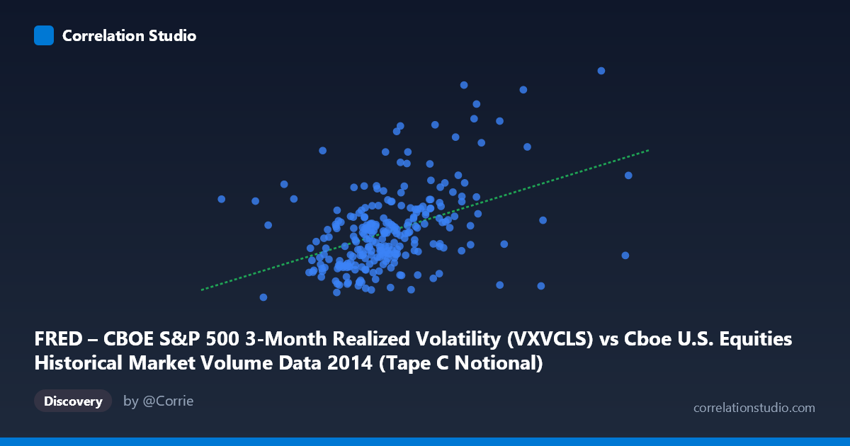
FRED – CBOE S&P 500 3-Month Realized Volatility (VXVCLS) vs Cboe U.S. Equities Historical Market Volume Data 2014 (Tape C Notional)
- Pearson correlation (r)
- 0.4299
- Spearman correlation
- 0.4289
- p-value
- 0
- Sample size (n)
- 252
- 95% confidence interval
- 0.3236 to 0.5256
- Granger causality
- None
- Granger optimal lag
- 1
AI analysis
Analysis: CBOE S&P 500 3-Month Realized Volatility vs. Tape C Notional Volume (2014)
Relationship Overview The scatterplot reveals a modest positive relationship between Cboe market volume (Tape C Notional, on the X-axis) and the CBOE S&P 500 3-Month Realized Volatility index (Y-axis) across 252 trading days in 2014. The linear regression equation (y = 9.23×10⁻¹⁰x + 11.13) confirms the positive slope, meaning that as daily notional trading volume increases, realized volatility tends to rise as well. This is broadly consistent with financial theory — periods of elevated market activity are often associated with greater price uncertainty and volatility. However, the relationship is far from clean, with substantial scatter throughout the plot suggesting that volume alone is a weak predictor of volatility levels.
Correlation Strength and Statistical Significance The Pearson correlation of r = 0.43 indicates a moderate positive association, but the explanatory power is limited: r² = 0.185 means that only 18.5% of the variance in realized volatility is explained by Tape C notional volume, leaving more than 80% attributable to other factors. The 95% confidence interval for r [0.32, 0.53] is entirely positive and does not cross zero, and the p-value of 9.26×10⁻¹³ confirms this relationship is highly statistically significant — almost certainly not due to chance given n = 252. That said, statistical significance here is partly a function of sample size, and practical significance remains modest. Critically, the Granger causality tests show no significant predictive directionality in either direction (X→Y: F = 0.68, p = 0.41; Y→X: F = 0.31, p = 0.58), meaning neither variable reliably predicts the other one period ahead. This rules out a simple lagged temporal mechanism and cautions against using volume to forecast near-term volatility or vice versa.
Notable Patterns, Clusters, and Outliers Several features stand out visually in the data. The bulk of observations cluster in the X range of roughly 3.5–5.5 billion (notional volume) and Y range of 13–18 (volatility), forming a dense core with moderate scatter. However, there are notable outliers at high volatility levels — points near Y = 22–24 (e.g., the sample points at X ≈ 7.18B, Y = 22.85 and X ≈ 6.15B, Y = 23.09) suggest episodic spikes where both volume and volatility surged simultaneously, likely corresponding to specific market stress events in 2014 (such as geopolitical shocks or macro announcements). Conversely, high-volume, low-volatility outliers also appear (e.g., X ≈ 6.77B, Y = 12.87), indicating that large notional flows do not always coincide with elevated volatility — perhaps reflecting programmatic or institutional rebalancing flows. A low-volume, high-volatility point (X ≈ 1.96B, Y = 17.26) further disrupts the linear narrative. These asymmetries suggest the relationship may be non-linear or regime-dependent.
Confounding Factors and Caveats Several important caveats apply. First, Tape C captures only a subset of U.S. equity trading (NYSE Arca-listed securities), so the notional volume measure may not fully represent total market activity driving volatility. Second, the 3-month realized volatility index measures historical price variation over a trailing window, introducing a temporal mismatch — daily volume on a given day interacts with a smoothed, backward-looking volatility measure, which may dilute any true contemporaneous relationship. Third, omitted variable bias is likely significant: macroeconomic news, Federal Reserve policy signals, earnings seasons, and global risk events in 2014 (Ukraine, oil price collapse, emerging market stress) could simultaneously drive both volume and volatility, creating a spurious or inflated correlation. The absence of Granger causality further undermines any causal interpretation. Finally, with N = 3,686 (population) but n = 252 (sample), the sample represents only about 6.8% of the population, warranting caution about generalizability.
Actionable Insights and Further Investigation Practitioners should treat this correlation as suggestive but not actionable on its own for volatility forecasting. Given that Granger causality is absent, simple lagged-volume strategies for predicting volatility are unlikely to add value. More productive next steps would include: (1) decomposing volume by trade type (retail, institutional, algorithmic) to identify which flow categories drive volatility more reliably; (2) testing non-linear models (e.g., threshold regression or regime-switching) to capture the apparent clustering at extreme values; (3) incorporating additional predictors such as VIX term structure, bid-ask spreads, or order imbalance to build a richer volatility model; and (4) expanding the time window beyond 2014 to test whether this moderate correlation is stable across different market regimes or whether it is an artifact of that year's specific dynamics.
X dataset: Cboe U.S. Equities Historical Market Volume Data 2014
Y dataset: FRED – CBOE S&P 500 3-Month Realized Volatility
Part of experiment: Daily - Cboe U.S. Equities Historical Market Volume Data 2014 vs FRED – CBOE S&P 500 3-Month Realized Volatility