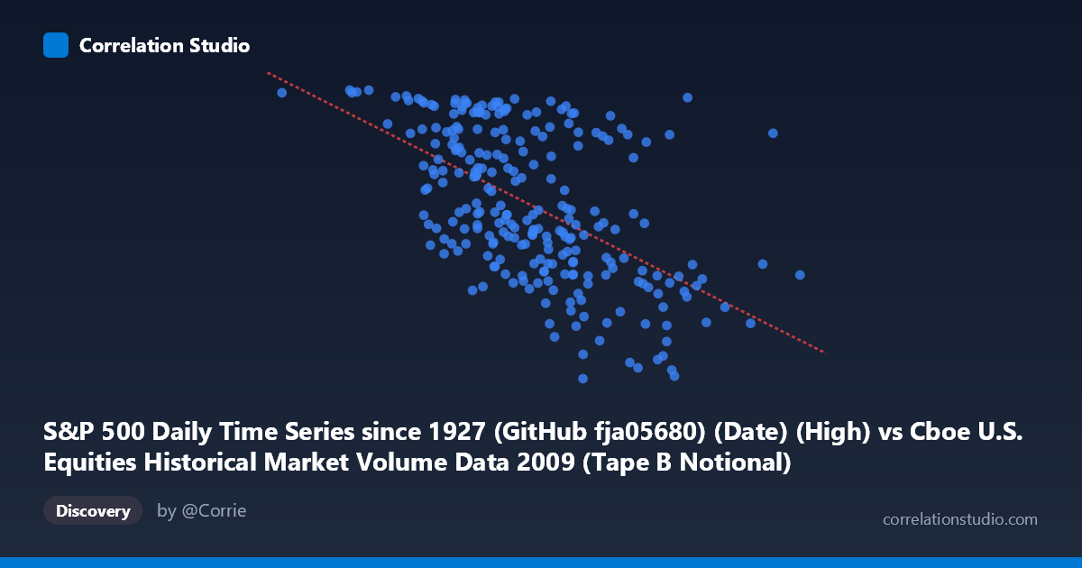
S&P 500 Daily Time Series since 1927 (GitHub fja05680) (Date) (High) vs Cboe U.S. Equities Historical Market Volume Data 2009 (Tape B Notional)
- Pearson correlation (r)
- -0.556
- Spearman correlation
- -0.57
- p-value
- 0
- Sample size (n)
- 252
- 95% confidence interval
- -0.6359 to -0.4643
- Granger causality
- X → Y
- Granger optimal lag
- 10
AI analysis
Analysis: S&P 500 Daily Highs vs. Cboe Tape B Notional Volume (2009)
Relationship Overview The scatterplot reveals a moderate negative relationship between the S&P 500 daily high price (X-axis) and Cboe Tape B notional trading volume (Y-axis) across 2009 trading days. As the S&P 500 daily high increases — broadly representing market price levels recovering through the year — Tape B notional volume tends to decline. This is visually consistent with the well-documented phenomenon of elevated trading volumes during periods of market stress and low prices (early 2009 bear market lows) contrasting with calmer, lower-volume conditions as prices recovered later in the year. The linear regression equation y = -4.79e-08x + 1209.22 quantifies this inverse slope, with the negative coefficient confirming the downward trend.
Correlation Strength and Statistical Significance The Pearson correlation of r = -0.556 indicates a moderate negative association, but the explained variance — r² = 0.309 — tells a more sobering story: only about 30.9% of the variance in Tape B notional volume is explained by the S&P 500 daily high. Nearly 70% of volume variation is driven by other factors. The 95% confidence interval of [-0.636, -0.464] is meaningfully narrow and entirely negative, confirming the direction is reliable, and the p-value of essentially zero at n=252 leaves no doubt this correlation is statistically significant rather than a sampling artifact. The Granger causality result adds an important temporal dimension: X (S&P 500 high) unidirectionally Granger-causes Y (Tape B notional) at an optimal lag of 10 periods (F=1.96, p=0.039), while the reverse direction fails significance (p=0.051). This suggests that S&P 500 price levels have modest predictive utility for near-future notional volume, though the effect is marginal and the F-statistic is not large.
Patterns, Clusters, and Outliers The sample points reveal notable heteroscedasticity: at lower X values (roughly 1.3B–3.5B range, corresponding to early 2009 depressed price levels), Y values cluster tightly at high notional volumes (1050–1130 range), while at higher X values (6B–9.5B, reflecting recovery), the Y values are more dispersed and span a wider range (700–1100). Several outliers are visible: the point near (1,320,771,983, 1126.48) sits in an extreme low-price, high-volume corner and likely corresponds to the post-crash volatility of early January 2009. Points like (7,526,902,255, 699.09) and (8,730,419,234, 778.69) represent high-price, low-volume sessions typical of the quieter late-2009 recovery. The scatter also shows a non-linear hint — the relationship may be better described by a curve that steepens at low X values — suggesting a linear model may underfit the true dynamic.
Confounding Factors and Caveats Several important caveats apply. First, this correlation is largely temporal in disguise: both variables are time-indexed through 2009, and the negative correlation may simply reflect the chronological arc of the year — markets were low and volatile in Q1 (high volume, low prices) and recovered by Q4 (lower volume, higher prices). This means the apparent X→Y relationship could be spurious co-movement driven by shared time trends rather than a direct causal mechanism between price levels and notional volume. Second, Tape B notional volume specifically covers NYSE American (AMEX) and regional exchange-listed securities, not the full market, so it may not respond identically to S&P 500 movements as broad market volume would. Third, the Granger causality result is borderline — p=0.039 barely clears the 0.05 threshold — warranting caution about over-interpreting the predictive direction.
Actionable Insights and Further Investigation Practitioners should detrend both series before drawing causal conclusions — removing the shared 2009 time trend via differencing or deseasonalization would reveal whether the relationship persists beyond the chronological arc. It would be valuable to extend this analysis across multiple years (e.g., 2007–2012) to test whether the inverse price-volume relationship holds in bull markets, bear markets, and recovery phases independently. Investigating implied volatility (VIX) as a mediating variable is strongly recommended, as fear-driven volatility likely explains much of the residual 69% variance. Finally, given the 10-day Granger lag, a rolling window regression could test whether this predictive relationship strengthens during high-volatility regimes, potentially offering a useful signal for market microstructure modeling or liquidity forecasting.
X dataset: Cboe U.S. Equities Historical Market Volume Data 2009
Y dataset: S&P 500 Daily Time Series since 1927 (GitHub fja05680) (Date)
Part of experiment: Daily - Cboe U.S. Equities Historical Market Volume Data 2009 vs S&P 500 Daily Time Series since 1927 (GitHub fja05680) (Date)