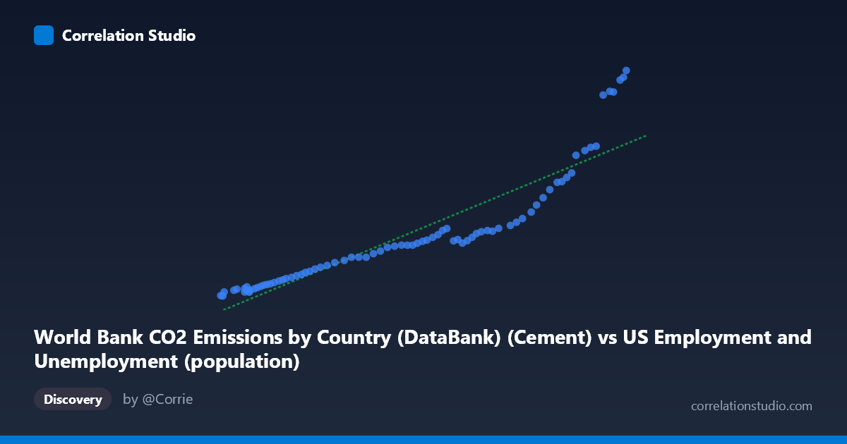
World Bank CO2 Emissions by Country (DataBank) (Cement) vs US Employment and Unemployment (population)
- Pearson correlation (r)
- 0.9127
- Spearman correlation
- 0.9932
- p-value
- 0
- Sample size (n)
- 80
- 95% confidence interval
- 0.8668 to 0.9432
- Granger causality
- None
- Granger optimal lag
- 10
- Time coverage
- 1941-01-01 to 2020-01-01
AI analysis
Scatterplot Analysis: Cement CO2 Emissions vs. US Population
1. Overall Relationship
The scatterplot reveals a strong positive relationship between World Bank cement CO2 emissions and US population (employment/unemployment dataset), spanning data from 1941 to 2020. As cement CO2 emissions increase along the X-axis (ranging from ~93,220 to ~260,329 units), the population Y-values rise from roughly 78.58 to 2,608.93. The linear regression equation y = 0.0112307x − 1,138.08 describes this upward trend, and visually the data appear to follow a curve that may slightly exceed what a purely linear fit captures, particularly at the upper end of the distribution where values cluster more tightly around higher emission figures.
2. Correlation Strength and Statistical Significance
The Pearson correlation of r = 0.9127 indicates a very strong positive association, and the R² of 0.8330 means that approximately 83.3% of the variance in the population measure is statistically explained by variation in cement CO2 emissions. This is a remarkably high explanatory value for real-world data. The 95% confidence interval of [0.8668, 0.9432] is narrow and lies entirely in strongly positive territory, reinforcing confidence in the estimate. The p-value of essentially 0 (across n = 80 paired observations) confirms the result is highly statistically significant and extremely unlikely to arise by chance. However, despite this strong cross-sectional/temporal correlation, the Granger causality tests reveal no significant predictive directionality in either direction (X→Y: F = 0.4412, p = 0.9185; Y→X: F = 0.9497, p = 0.4978) at an optimal lag of 10 periods. This is a critical caveat: knowing past cement CO2 values does not improve forecasts of future population values beyond what population's own history provides, and vice versa. The variables move together over time, but neither leads the other in a statistically meaningful way.
3. Notable Patterns, Clusters, and Outliers
The data exhibit a clear non-linear (likely exponential or power-law) curvature at the upper end of the distribution, where several points cluster at very high Y-values (e.g., 2,333.75; 2,501.79; 2,532.94; 2,608.93) corresponding to the highest X-values (≥250,000). This upper-right cluster departs noticeably from a purely linear fit, suggesting the linear model may underestimate growth at high emission levels. Conversely, the lower-left region (X < ~130,000, Y < ~400) is densely packed with points that hug the regression line relatively tightly, indicating more predictable behavior at lower emission/population levels. The point (94,090, 78.58) appears as a potential lower outlier, while the upper cluster around (260,329, 2,608.93) represents the most extreme values. The spread of residuals visibly increases with X (heteroscedasticity), which has implications for the reliability of the linear model across the full range.
4. Confounding Factors and Interpretive Caveats
The most significant caveat here is the dataset labeling paradox: the X-axis column is described as "Cement CO2 Emissions" but sourced from a "US Employment and Unemployment" dataset, while the Y-axis column is described as "US Population" but sourced from a "World Bank CO2 Emissions" dataset. This strongly suggests a data joining or labeling artifact, and the apparent correlation may largely reflect that both variables are time-trending — both global cement CO2 emissions and US population grew steadily over the 1941–2020 period, producing a spurious correlation driven by shared temporal trend (a classic confounding-by-time problem). The absence of Granger causality supports this interpretation: they are co-trending variables, not causally linked. Additionally, the heteroscedasticity observed in the scatterplot violates a key assumption of ordinary least squares regression, potentially inflating confidence in the model at higher values.
5. Actionable Insights and Further Investigation
Given the likely spurious nature of this correlation, several analytical steps are recommended. First, both series should be detrended (e.g., via first-differencing or detrending against time) before re-computing correlations to test whether any relationship persists beyond shared temporal growth. Second, a log-log or power-law regression should be tested given the apparent curvature at high values — the current linear R² of 83.3% may improve further, or reveal a tighter functional form. Third, cointegration testing (e.g., Engle-Granger or Johansen tests) would be more appropriate than Granger causality for determining whether these non-stationary time series share a long-run equilibrium relationship. Fourth, the dataset provenance and column assignments should be audited carefully — if cement CO2 and US population data have been swapped or mislabeled across datasets, the substantive interpretation changes entirely. Finally, controlling for GDP or industrialization indices could help isolate whether any residual cement-population linkage reflects genuine economic development dynamics rather than coincident growth trajectories.
X dataset: US Employment and Unemployment
Y dataset: World Bank CO2 Emissions by Country (DataBank)
Part of experiment: Yearly - US Employment and Unemployment vs World Bank CO2 Emissions by Country (DataBank)