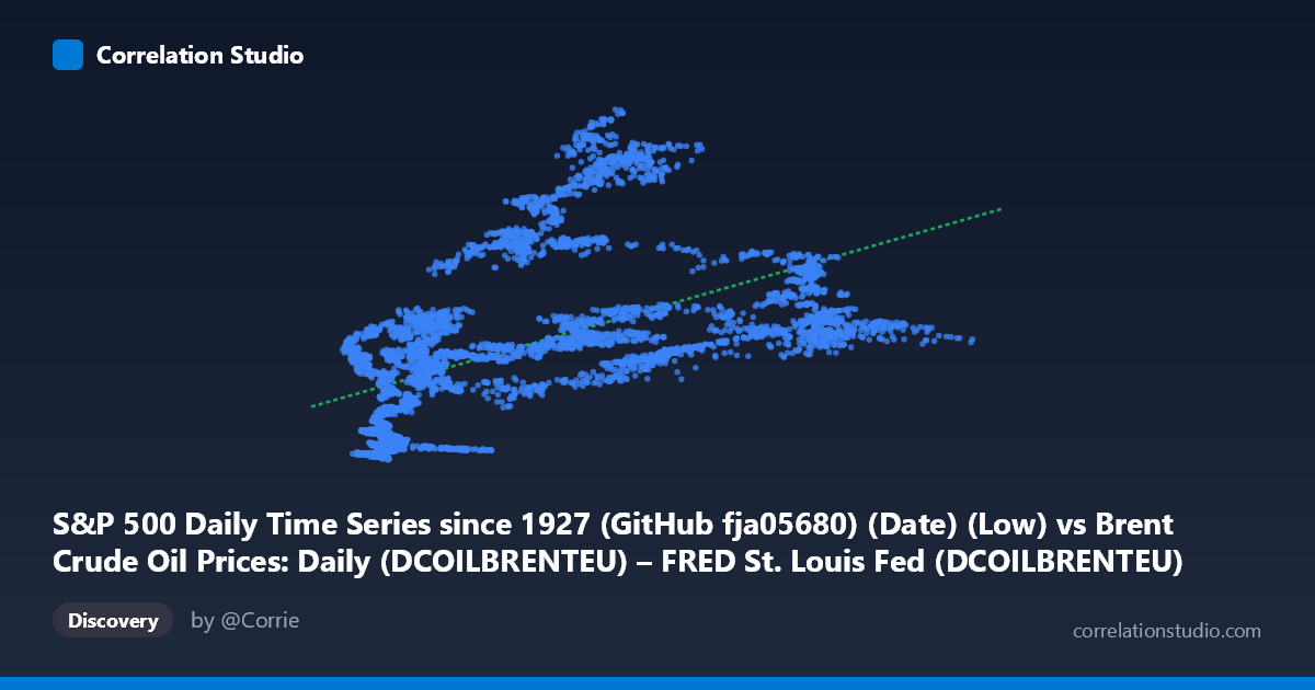
S&P 500 Daily Time Series since 1927 (GitHub fja05680) (Date) (Low) vs Brent Crude Oil Prices: Daily (DCOILBRENTEU) – FRED St. Louis Fed (DCOILBRENTEU)
- Pearson correlation (r)
- 0.5375
- Spearman correlation
- 0.6919
- p-value
- 0
- Sample size (n)
- 8140
- 95% confidence interval
- 0.5219 to 0.5528
- Granger causality
- None
- Granger optimal lag
- 1
AI analysis
Brent Crude Oil Price vs. S&P 500: Correlation Analysis
1. What the Visualization Reveals
The scatterplot depicts the relationship between the S&P 500 daily low prices (X-axis) and Brent Crude Oil spot prices (Y-axis) across a 32-year period from May 1987 to December 2019. The overall pattern shows a broad, upward-trending cloud of data points, indicating that higher S&P 500 levels tend to coincide with higher crude oil prices. However, the substantial vertical scatter at virtually every X-value immediately signals that this relationship is far from deterministic — at any given S&P 500 level, Brent crude prices span enormous ranges, sometimes differing by $1,500–$2,000+ per barrel equivalent in index terms. This visual diffuseness is the dominant feature of the chart.
2. Correlation Strength, Direction, and Temporal Predictability
The Pearson correlation of r = 0.5375 indicates a moderate positive relationship, but the explanatory power is modest: R² = 0.289, meaning the S&P 500 daily low explains only ~28.9% of the variance in Brent crude prices. Roughly 71% of crude price variation is driven by factors entirely outside this relationship. The 95% confidence interval of [0.5219, 0.5528] is narrow given the large paired sample (n = 8,140), confirming the correlation estimate is statistically stable and not an artifact of sampling. The p-value of effectively zero confirms this correlation is highly unlikely to be chance — but statistical significance here should not be confused with practical or causal significance. Critically, the Granger causality tests fail in both directions (X→Y: F = 0.94, p = 0.33; Y→X: F = 0.87, p = 0.35), meaning neither variable meaningfully predicts the other at a one-period lag. This is a pivotal finding: despite co-movement, neither series leads the other temporally, ruling out simple predictive trading strategies in either direction.
3. Notable Patterns, Clusters, and Non-Linear Features
Several structural features stand out in the data. There is a dense cluster at lower X-values (roughly S&P 500 lows below 40), corresponding to the pre-2000 period when both the index and oil prices were at historically lower levels. Above X ≈ 60–70, the data fans out considerably, with oil prices ranging from below $1,000 to above $3,000, reflecting the high-volatility era of 2000–2019 including the commodity supercycle, the 2008 financial crisis, and subsequent shale-driven price collapses. The Spearman ρ exceeding Pearson r is a critical diagnostic: it suggests the relationship is non-linear, likely logarithmic or following a power curve, where early gains in the S&P 500 correspond to proportionally larger oil price increases, with diminishing sensitivity at higher index levels. A polynomial or logarithmic regression model would almost certainly improve fit meaningfully over the linear model (y = 11.47x + 645.96).
4. Confounding Factors and Caveats
This correlation almost certainly reflects shared exposure to a common driver — global economic growth — rather than any direct causal mechanism between equity prices and crude oil. Both assets tend to rise during economic expansions (rising industrial demand, risk appetite) and fall during recessions, creating spurious co-movement. Time-series non-stationarity is a major concern: both series exhibit strong upward trends over three decades, and much of the measured correlation may simply reflect two trending variables moving together over time rather than a meaningful contemporaneous relationship. Currency effects (both priced in USD), geopolitical shocks (Gulf Wars, OPEC supply decisions, Iran sanctions), and the structural break introduced by the U.S. shale revolution post-2014 all represent confounders that shift the oil-equity relationship dramatically across sub-periods. The mixing of pre- and post-shale regimes in a single correlation coefficient is particularly problematic.
5. Actionable Insights and Further Investigation
Given these findings, several analytical paths would add significant value. Sub-period analysis (pre-2000, 2000–2008 commodity supercycle, 2009–2014 post-crisis recovery, 2014–2019 shale era) would likely reveal dramatically different correlation structures and potentially reverse the direction in some windows. Detrending both series (via first-differencing or percent returns) before computing correlation would eliminate the spurious trend-driven component and reveal whether true contemporaneous co-movement exists in price changes rather than price levels. Testing a logarithmic regression model (consistent with the Spearman Pearson signal) should be prioritized. Finally, incorporating lagged macro variables — global GDP growth, USD index, OPEC production data — as covariates in a multivariate model would help disentangle the genuine relationship from shared macro exposure, and might reveal whether crude or equities respond faster to common shocks even when neither directly Granger-causes the other.
X dataset: Brent Crude Oil Prices: Daily (DCOILBRENTEU) – FRED St. Louis Fed
Y dataset: S&P 500 Daily Time Series since 1927 (GitHub fja05680) (Date)
Part of experiment: Daily - Brent Crude Oil Prices: Daily (DCOILBRENTEU) – FRED St. Louis Fed vs S&P 500 Daily Time Series since 1927 (GitHub fja05680) (Date)