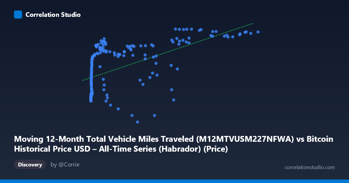
Moving 12-Month Total Vehicle Miles Traveled (M12MTVUSM227NFWA) vs Bitcoin Historical Price USD – All-Time Series (Habrador) (Price)
- Pearson correlation (r)
- 0.5576
- Spearman correlation
- 0.7186
- p-value
- 0
- Sample size (n)
- 188
- 95% confidence interval
- 0.4504 to 0.6489
- Granger causality
- None
- Granger optimal lag
- 10
AI analysis
Analysis: Bitcoin Price vs. Vehicle Miles Traveled
1. What the Visualization Reveals
This scatterplot juxtaposes Bitcoin's historical USD price against the 12-month rolling total of US vehicle miles traveled (VMT). At face value, the data show a moderate positive correlation, but this is almost certainly a spurious relationship driven by shared time trends rather than any causal or economically meaningful link. Both series have generally risen over the 2010–2026 window (Bitcoin due to adoption/speculation cycles, VMT due to population growth and post-COVID recovery), which mechanically produces co-movement even absent any real interaction.
2. Strength, Direction, and Statistical Interpretation
The Pearson correlation (r = 0.558, r² = 0.311) indicates that only about 31% of the variance in Bitcoin price is "explained" by VMT — leaving nearly 70% unaccounted for. The 95% CI [0.450, 0.649] is reasonably tight and excludes zero, and the p-value rounds to 0, so the correlation is statistically significant in a naive sense. However, statistical significance here should not be mistaken for practical or causal significance: with N=188 paired points drawn from trending time series, autocorrelation inflates apparent significance, and the p-value doesn't account for the non-stationarity of either series.
Critically, the Granger causality tests show no predictive direction in either direction (X→Y: p=0.74; Y→X: p=0.75). This is a strong signal that neither series helps forecast the other once lag structure is considered — undermining any narrative that vehicle travel trends drive Bitcoin prices or vice versa. Combined with the note that Spearman ρ exceeds Pearson r, the relationship is likely nonlinear/monotonic (e.g., logarithmic), consistent with Bitcoin's exponential-then-plateauing price trajectory versus VMT's slower, smoother growth.
3. Notable Patterns and Features
- Clustering by regime: Low-X, low-Y points dominate (Bitcoin under ~$1,000 with VMT in the 2.9–3.0M range) — this reflects the 2010–2013 era. High-X, high-Y points (Bitcoin $50,000, VMT 3.2M) reflect 2020s bull markets. - Vertical scatter at low X: Many points cluster near X≈0–20 with wildly varying Y (2,832,198 to over 3,000,000), showing Bitcoin's price was near-zero for a long stretch while VMT moved independently — a sign the "relationship" is really just two unrelated clocks ticking. - Nonlinear curvature: The pattern resembles a logarithmic or power-law shape (rapid Y change at very low X, flattening at high X), matching the analysis note about Spearman Pearson. - A likely outlier: (45092.81, 2867625.00) — high Bitcoin price paired with an anomalously low VMT — breaks the general upward trend, possibly a COVID-period data point where VMT collapsed while Bitcoin was rallying.
4. Confounding Factors and Caveats
This is a textbook case of spurious correlation via common trend/time confound. Both variables are non-stationary and increasing over the sample period for entirely unrelated structural reasons: Bitcoin due to adoption, halving cycles, and speculative demand; VMT due to demographic growth, economic activity, and (recently) COVID-related disruption and recovery. Neither has a plausible causal mechanism linking it to the other. Additional caveats: - Mismatched frequency/smoothing (rolling 12-month VMT vs. daily/point Bitcoin price) can introduce artificial smoothness and lag artifacts. - The dataset spans very different Bitcoin volatility regimes (multiple boom-bust cycles) not mirrored in VMT, meaning the linear fit is heavily influenced by a handful of high-X bull-market points. - No adjustment for inflation, population growth, or detrending was applied — a spurious-regression risk when both series are trending.
5. Suggestions for Further Investigation
- Detrend or difference both series (e.g., use % month-over-month changes rather than levels) and recompute correlation — this is the standard remedy for spurious trend-driven correlation and would likely show r near zero. - Test for cointegration (e.g., Engle-Granger) rather than relying on simple Pearson/Granger-on-levels, since both series are likely unit-root processes. - Fit a log-log or log-linear model given the Spearman/Pearson divergence, and re-assess r². - Treat this pairing primarily as a demonstration of confounding-by-time-trend rather than a genuine economic relationship — VMT is not a meaningful predictor of Bitcoin price, and the analysis should pivot to variables with a plausible causal link (e.g., monetary policy, crypto exchange volume, or macro liquidity indices).
X dataset: Bitcoin Historical Price USD – All-Time Series (Habrador)
Y dataset: Moving 12-Month Total Vehicle Miles Traveled
Part of experiment: Bitcoin - Bitcoin Historical Price USD – All-Time Series (Habrador) vs Moving 12-Month Total Vehicle Miles Traveled