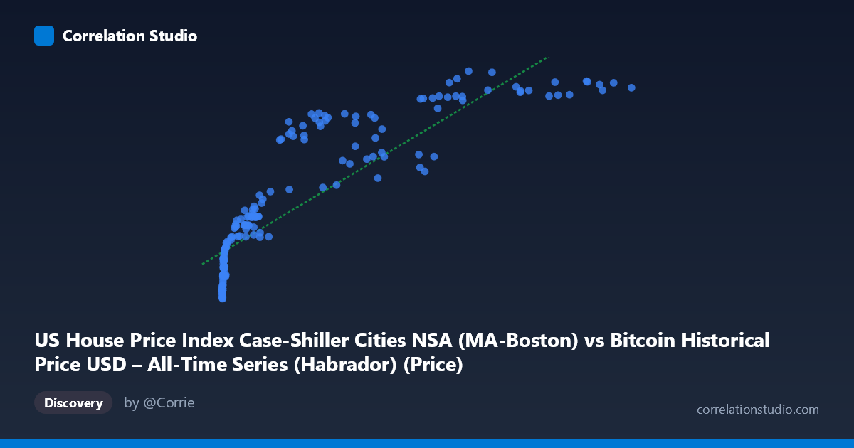
US House Price Index Case-Shiller Cities NSA (MA-Boston) vs Bitcoin Historical Price USD – All-Time Series (Habrador) (Price)
- Pearson correlation (r)
- 0.8717
- Spearman correlation
- 0.971
- p-value
- 0
- Sample size (n)
- 191
- 95% confidence interval
- 0.8328 to 0.902
- Granger causality
- None
- Granger optimal lag
- 9
- Time coverage
- 2010-08-01 to 2026-06-01
- Recomputed on refreshed data
- 2026-10-24 (r was 0.8671)
AI analysis
Analysis: Bitcoin Price vs. Boston Case-Shiller Home Price Index
1. What the Visualization Reveals
The scatterplot shows a strong positive association between Bitcoin's historical USD price and the Boston Case-Shiller Home Price Index, but the relationship is clearly non-linear. At low Bitcoin values (under ~$1,000), the Case-Shiller index is compressed in a narrow band (roughly 145–200), while Bitcoin itself spans several orders of magnitude in this same region. As Bitcoin climbs into the tens of thousands, the home price index rises more steadily into the 250–350 range. This pattern — a steep initial compression followed by a more linear climb — is the classic signature of a logarithmic or power-law relationship rather than a straight line, which is reinforced by the note that Spearman's ρ exceeds Pearson's r.
2. Strength, Direction, and Statistical Meaning
The Pearson correlation (r = 0.863) is strong and positive, with r² indicating that 74.5% of the variance in the home price index is statistically associated with Bitcoin's price level (or vice versa) under a linear model. The 95% CI [0.821, 0.896] is tight and the p-value is effectively 0, meaning the correlation is highly unlikely to be a sampling artifact — it's a robust statistical relationship. However, statistical association is not evidence of a causal or predictive relationship. The Granger causality tests are decisive here: neither direction (X→Y or Y→X) shows significant predictive power (p = 0.68 and p = 0.79, respectively). This means Bitcoin's past values do not help forecast future Case-Shiller values, and vice versa — despite the strong contemporaneous correlation, neither series temporally "leads" the other in a statistically detectable way.
3. Notable Patterns and Features
- Compression at low X: Dozens of points cluster near X < 1,000 with Y values tightly packed between 145–220, indicating Bitcoin's early years (2010–2013) coincided with a relatively flat/recovering housing market post-2008 crash. - Divergence at high X: At the highest Bitcoin values ($100,000), Y plateaus near 340–354, suggesting the home price index may be saturating while Bitcoin continues to swing wildly (note the extreme X range: 0.06 to 118,670). - No visible cyclical reversals: Despite Bitcoin's well-known boom-bust cycles (2013, 2017, 2021 crashes), the Case-Shiller index shows no corresponding whipsaw — it rises steadily, reflecting its slower-moving, less volatile nature. - Curvature: The overall shape looks concave (log-like) — consistent with the suggestion that a log-transformed X or polynomial fit would outperform the linear model.
4. Confounding Factors and Caveats
This is a textbook case of spurious correlation via shared trend, not a meaningful economic relationship: - Both series are non-stationary time series that trended upward over the same 2010–2026 window due to entirely different macro drivers (housing market recovery/QE-era low rates for Case-Shiller; adoption/speculation cycles for Bitcoin). - The correlation is likely driven by mutual correlation with time/macro liquidity conditions (e.g., near-zero interest rates 2010–2021, quantitative easing, inflation post-2020) rather than any direct link between crypto markets and Boston real estate. - The Granger test result confirms this suspicion: if there were a genuine causal pathway (e.g., crypto wealth effects flowing into home purchases), we'd expect at least weak lead-lag predictability. Its absence supports the "common trend" explanation over a causal one. - Case-Shiller is monthly and smoothed; Bitcoin is highly volatile daily — the mismatch in volatility/frequency inflates apparent correlation when both are simply trending over multi-year windows.
5. Actionable Insights
- Do not use this correlation for trading or investment decisions (e.g., "Bitcoin predicts home prices") — the Granger results explicitly rule out predictive value in either direction. - Detrend both series first (e.g., using year-over-year % change or differencing) and recompute correlation; this is the standard way to check if the relationship survives once the shared time-trend is removed. It's likely r will drop substantially. - Try a log-log or log-linear model for X, given the log-normal appearance of Bitcoin's distribution and the noted non-linearity — this should improve fit and offer more interpretable elasticities. - Introduce a common macro covariate (interest rates, M2 money supply, or CPI) as a control variable to test whether the Bitcoin–housing correlation vanishes once liquidity conditions are accounted for — this would help distinguish genuine co-movement from confound-driven trend correlation.
X dataset: Bitcoin Historical Price USD – All-Time Series (Habrador)
Y dataset: US House Price Index Case-Shiller Cities NSA
Part of experiment: Bitcoin - Bitcoin Historical Price USD – All-Time Series (Habrador) vs US House Price Index Case-Shiller Cities NSA