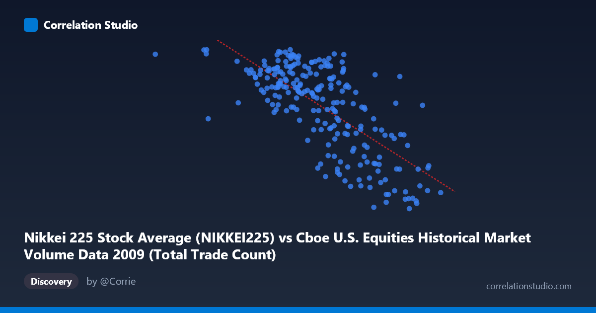
Nikkei 225 Stock Average (NIKKEI225) vs Cboe U.S. Equities Historical Market Volume Data 2009 (Total Trade Count)
- Pearson correlation (r)
- -0.7167
- Spearman correlation
- -0.6804
- p-value
- 0
- Sample size (n)
- 235
- 95% confidence interval
- -0.7737 to -0.6482
- Granger causality
- None
- Granger optimal lag
- 10
AI analysis
Scatterplot Analysis: Nikkei 225 vs. U.S. Equities Total Trade Count (2009)
Relationship Overview
The scatterplot reveals a moderately strong negative relationship between the Nikkei 225 Stock Average and U.S. Equities Total Trade Count throughout 2009. As the Nikkei 225 index values increase, U.S. equity trade counts tend to decline, and vice versa. The linear regression equation (y = -0.00117x + 12,485) captures this inverse trend, suggesting that higher Japanese equity valuations coincide with reduced trading activity volume on U.S. exchanges. This pattern is visually apparent across the full X range of roughly 630,000 to 4,134,000, with higher trade counts clustering at lower Nikkei values and lower trade counts appearing as Nikkei values rise.
Correlation Strength and Statistical Significance
The correlation coefficient of r = -0.717 indicates a moderately strong negative association, and the R² of 0.514 means that approximately 51.4% of the variance in U.S. trade counts is statistically explained by Nikkei 225 levels — a meaningful but incomplete explanation, leaving nearly half the variance attributable to other factors. The 95% confidence interval of [-0.774, -0.648] is relatively narrow and does not cross zero, lending confidence to the direction and approximate magnitude of the relationship. With a p-value reported as effectively 0 across an N of 3,232, the correlation is highly statistically significant and almost certainly not a chance finding. However, Granger causality tests tell a more cautious story: neither direction (X→Y nor Y→X) reaches significance at the optimal 10-period lag (F = 1.46, p = 0.155 and F = 1.44, p = 0.164 respectively), meaning the data provide no reliable evidence that one variable temporally predicts the other. The correlation is real, but directionality and causation remain unestablished.
Notable Patterns and Outliers
Several features stand out in the sample points. There is a visible cluster of high trade counts (Y 10,000) concentrated in the lower-to-mid Nikkei range (roughly 1,800,000–2,700,000), consistent with the early 2009 period when markets were volatile and heavily traded during crisis conditions. Conversely, as Nikkei values exceed ~3,200,000–3,700,000, trade counts drop noticeably toward the 7,000–8,500 range, reflecting the calmer, recovering market environment later in the year. A few potential outliers are visible — notably points with very high trade counts (10,500) at mid-range Nikkei values and some low trade counts (~7,054–7,500) at the highest Nikkei readings — which may reflect specific market events or anomalous trading sessions. The scatter does not suggest a strongly non-linear relationship, though slight heteroscedasticity (wider spread at lower Nikkei values) is plausible.
Confounding Factors and Caveats
This correlation almost certainly reflects a shared temporal driver rather than a direct causal link between Japanese equity prices and U.S. trade volumes. Both variables are strongly influenced by the 2009 global financial crisis recovery trajectory: early 2009 saw market lows, extreme fear, and frenetic trading activity, while later 2009 saw stabilization, rising equity prices worldwide (including the Nikkei), and declining but normalizing trade volumes. This creates a classic spurious correlation via common cause — the macroeconomic environment simultaneously drove both series in opposite directions. Additionally, the axes appear to involve unit scaling (Nikkei values in the millions range seem unusual for an index that trades around 7,000–10,000 points), suggesting the X-axis may represent a derived or transformed Nikkei-related variable (possibly notional value or a composite), which warrants clarification before interpretation. The dataset and column label assignments also appear potentially swapped in the axis metadata, which should be verified.
Actionable Insights and Further Investigation
Given the strong contemporaneous correlation but absent Granger causality, the most productive next step would be to introduce explicit time controls — such as including a time trend variable or month fixed effects — to determine how much of the correlation dissolves once the shared crisis-recovery trajectory is accounted for. Analysts should also investigate whether VIX (volatility index) or other fear/risk indicators serve as the true common driver mediating both series. It would be worthwhile to examine whether this negative relationship persists in other years (2010–2015), or whether it is unique to the extraordinary 2009 environment. Finally, clarifying the exact nature of the X variable (raw Nikkei levels vs. a volume-weighted or notional construct) and confirming axis assignments would be essential before drawing any policy or trading conclusions from this relationship.
X dataset: Cboe U.S. Equities Historical Market Volume Data 2009
Y dataset: Nikkei 225 Stock Average
Part of experiment: Daily - Cboe U.S. Equities Historical Market Volume Data 2009 vs Nikkei 225 Stock Average