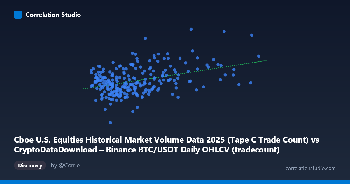
Cboe U.S. Equities Historical Market Volume Data 2025 (Tape C Trade Count) vs CryptoDataDownload – Binance BTC/USDT Daily OHLCV (tradecount)
- Pearson correlation (r)
- 0.401
- Spearman correlation
- 0.2799
- p-value
- 0
- Sample size (n)
- 250
- 95% confidence interval
- 0.2914 to 0.5001
- Granger causality
- None
- Granger optimal lag
- 10
AI analysis
Analysis: Cboe Equities Trade Count vs. Binance BTC/USDT Trade Count
1. Overview of the Relationship
The scatterplot displays a modest positive association between two seemingly unrelated market activity metrics: U.S. equities trade counts (Cboe, mislabeled as X but described as such) and Binance BTC/USDT trade counts. The data cloud shows a loose upward drift — as X increases, Y tends to increase slightly — but the dispersion is wide, with points scattered broadly around the regression line (y = 0.0897x + 2,355,680). The majority of X values cluster tightly between ~1.7M and ~5M, with a sparse tail of higher-X outliers extending to nearly 11.8M, giving the plot a "comet" shape rather than a tight linear band.
2. Strength, Direction, and Statistical Confidence
The correlation coefficient (r = 0.401) indicates a weak-to-moderate positive relationship. Critically, r² = 0.161 means only about 16% of the variance in Y is explained by X — the remaining 84% is driven by other factors entirely. The 95% CI [0.291, 0.500] is reasonably narrow and excludes zero, and the p-value (4.5×10⁻¹¹) confirms this correlation is highly statistically significant — it is very unlikely to be a product of sampling noise. However, statistical significance should not be conflated with practical strength: with n=250, even modest correlations become "significant," but the effect size here remains small. The Granger causality tests reinforce this: neither direction (X→Y or Y→X) shows significant predictive power (p = 0.98 and p = 0.65, respectively) at the optimal lag of 10 periods. This strongly suggests the two series do not temporally lead one another — the correlation is likely contemporaneous/coincidental or driven by a shared external factor, not a causal or predictive relationship in either direction.
3. Notable Patterns and Outliers
The scatter reveals a dense cluster of points in the lower-left region (X: 1.7M–4M, Y: 2M–3M trade counts), representing the bulk of "normal" trading days. A handful of high-X outliers (e.g., ~6.6M, ~7.5M, ~8.8M, ~9.8M) pull the regression slope upward but don't correspond to proportionally higher Y values — several high-X points still cluster around Y≈3M, similar to low-X points. This suggests the relationship may be driven disproportionately by a few extreme-volume days rather than a consistent trend across the full range, raising concern about leverage points skewing the fit. There's no evidence of a tight linear trend, exponential growth, or clear regime-switching pattern — just diffuse positive drift.
4. Confounding Factors and Caveats
Several caveats apply. First, both series are volume/activity metrics tied to overall market conditions — periods of macro volatility, risk-on/risk-off sentiment, or major news events could simultaneously inflate trading activity across both equities and crypto markets without one causing the other (a classic confound via a shared latent driver like "market-wide volatility" or "day-of-week/seasonality effects"). Second, these are time-series data (daily, 2025), meaning autocorrelation within each series (e.g., trends, weekday/weekend effects) could inflate the apparent cross-correlation — a spurious correlation risk common when regressing two non-stationary trending series. Third, the mismatched labels in the axis descriptions (Cboe data described under X but the OHLCV volume description appears swapped) suggest possible data-alignment issues worth double-checking before drawing conclusions.
5. Suggestions for Further Investigation
Given the weak r², lack of Granger causality, and potential confounding, this correlation should not be used for predictive trading or causal claims linking equities and crypto trade counts. Recommended next steps: (1) test for stationarity (ADF test) and consider differencing both series to rule out spurious trend-driven correlation; (2) introduce a third variable (e.g., VIX, overall crypto market cap, or macro news events) to check if it explains the shared variance better than a direct link; (3) examine the high-X outlier days individually — are they tied to specific market events (options expiry, ETF launches, etc.)? (4) Consider robust regression or removing leverage points to see if the r drops further, confirming whether the correlation is outlier-driven; (5) if a relationship is still of interest, explore non-linear or lagged specifications beyond the tested 10-period Granger window.
X dataset: CryptoDataDownload – Binance BTC/USDT Daily OHLCV
Y dataset: Cboe U.S. Equities Historical Market Volume Data 2025
Part of experiment: Bitcoin - CryptoDataDownload – Binance BTC/USDT Daily OHLCV vs Cboe U.S. Equities Historical Market Volume Data 2025