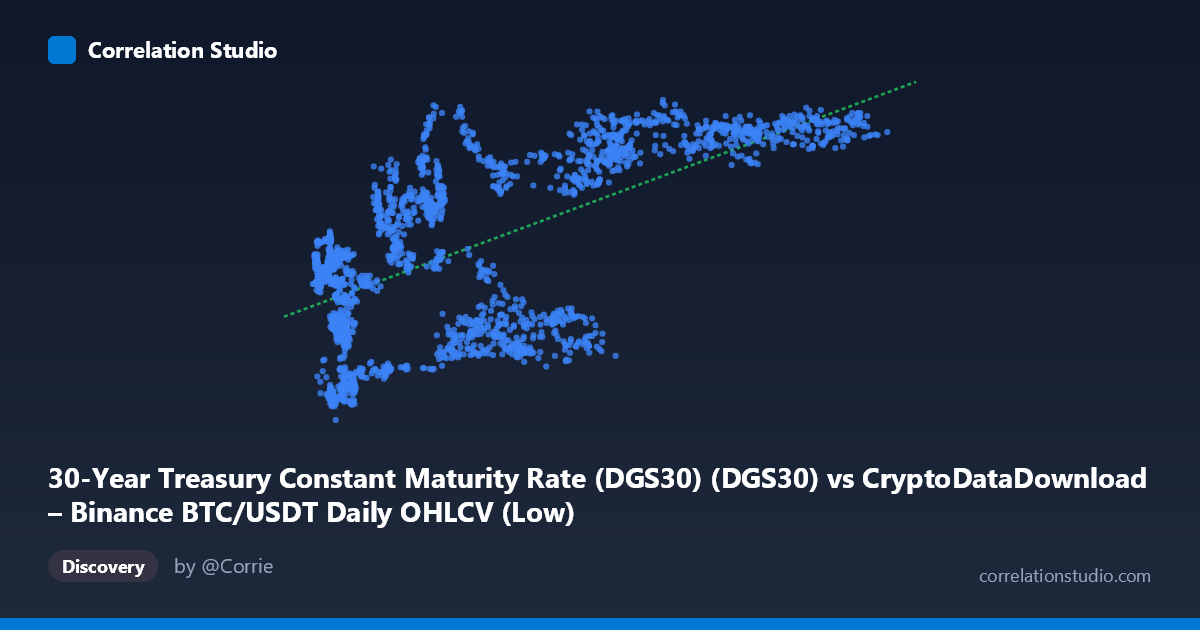
30-Year Treasury Constant Maturity Rate (DGS30) (DGS30) vs CryptoDataDownload – Binance BTC/USDT Daily OHLCV (Low)
- Pearson correlation (r)
- 0.6531
- Spearman correlation
- 0.5717
- p-value
- 0
- Sample size (n)
- 2197
- 95% confidence interval
- 0.6285 to 0.6765
- Granger causality
- None
- Granger optimal lag
- 1
AI analysis
Analysis: BTC/USDT Price vs. 30-Year Treasury Yield
Note on axis labeling: The metadata appears swapped — the described "X-axis" (labeled DGS30) actually contains large numeric values (2,817–123,084) consistent with BTC/USDT price data, while the "Y-axis" (labeled BTC Low) contains small values (0.99–5.18) consistent with treasury yields. The analysis below interprets the data as presented: X = BTC/USDT price, Y = 30-Year Treasury yield.
1. Relationship Overview
The scatterplot shows a moderate positive association between Bitcoin price and the 30-year Treasury yield. As BTC price rises from roughly $3,000 to $120,000+, the treasury yield trends upward from near 1% toward the 4.5–5% range. The relationship is not tightly linear — there's a visible "S-curve" or saturating pattern: yields cluster low (~1.5–2%) when BTC is under $20,000, then klimb steeply through the $20,000–$70,000 range, and plateau near 4.5–5% for BTC prices above $70,000.
2. Strength, Direction, and Statistical Confidence
The correlation coefficient (r = 0.653) indicates a moderate-to-strong positive relationship, with r² = 0.427 meaning only about 43% of the variance in treasury yields is explained by BTC price movements (or vice versa) — leaving the majority (57%) driven by other factors. The 95% CI [0.628, 0.677] is narrow, and p ≈ 0 confirms this correlation is highly statistically significant and not due to chance, given the large sample (n = 2,197). However, statistical significance should not be conflated with strong predictive power or causation. Critically, the Granger causality tests show no significant directional predictability in either direction (BTC→Yield: p = 0.067; Yield→BTC: p = 0.313). This suggests the correlation is likely driven by both series independently trending over the same macro period (2017–2026) rather than one variable temporally leading or causing changes in the other.
3. Notable Patterns and Outliers
Several structural features stand out: - Regime clustering: Data points form loose bands — a low-BTC/low-yield cluster (BTC < $20K, yield 1.3–3.5%), a middle transition zone with high scatter (BTC $20K–$60K, yield spanning 1.8–4.7%), and a high-BTC/high-yield plateau (BTC $70K, yield consistently 4.5–5%). - Vertical scatter in the mid-range: At similar BTC prices (~$40,000–$60,000), yields vary widely (1.87% to 4.74%), indicating BTC price alone poorly predicts yield in this zone — likely reflecting different time periods with similar BTC valuations but different macro regimes. - Yield ceiling effect: Yields appear capped near 5%, suggesting nonlinearity better modeled by a logarithmic or logistic curve than the fitted linear equation. - Low-BTC anomalies: A few points with BTC ~$6,000–$8,000 show elevated yields (2.6–3.3%) despite low price, breaking the general pattern — possibly reflecting different historical periods (e.g., 2018 vs. 2022 crashes) with divergent yield environments.
4. Confounding Factors and Caveats
This correlation is almost certainly spurious or indirect, driven by shared time-trend exposure rather than genuine economic linkage. Both BTC price and 30-year yields have risen over 2017–2026 due to entirely different macro forces: BTC's ascent reflects adoption, liquidity cycles, and speculative demand, while treasury yields reflect Fed policy, inflation expectations, and fiscal conditions. Since both variables are non-stationary time series trending upward over the same multi-year window, standard correlation is inflated by this shared temporal drift — a classic case of "spurious regression" risk. The lack of Granger causality reinforces that this is not a real predictive/causal relationship but coincidental co-trending.
5. Recommendations for Further Investigation
- Detrend or difference both series (e.g., use daily/monthly % changes rather than levels) and recompute correlation — this will likely reveal a much weaker or insignificant relationship, testing the spurious-regression hypothesis. - Segment by macro regime (e.g., pre/post-2022 rate hikes) to see if the relationship is regime-dependent rather than continuous. - Given the Granger results, do not use one series to forecast the other in a trading or planning context — the temporal linkage is not statistically supported. - Investigate a shared third factor (e.g., inflation expectations, real interest rates, or general market liquidity/risk appetite) that may simultaneously drive both series, using multivariate regression or a common macro-factor model instead of bivariate correlation.
X dataset: CryptoDataDownload – Binance BTC/USDT Daily OHLCV
Y dataset: 30-Year Treasury Constant Maturity Rate (DGS30)
Part of experiment: Bitcoin - CryptoDataDownload – Binance BTC/USDT Daily OHLCV vs 30-Year Treasury Constant Maturity Rate (DGS30)