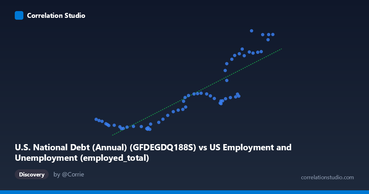
U.S. National Debt (Annual) (GFDEGDQ188S) vs US Employment and Unemployment (employed_total)
- Pearson correlation (r)
- 0.8728
- Spearman correlation
- 0.9037
- p-value
- 0
- Sample size (n)
- 60
- 95% confidence interval
- 0.7951 to 0.9223
- Granger causality
- None
- Granger optimal lag
- 10
AI analysis
Scatterplot Analysis: U.S. National Debt (% GDP) vs. Total Employment
1. Overall Relationship
The scatterplot reveals a strong positive relationship between U.S. National Debt as a percentage of GDP and total U.S. employment over the period 1966–2025. As national debt rises, total employment tends to increase as well. The linear regression equation (y = 0.000941932x − 51.2335) captures the general upward trend, though the scatter pattern suggests the relationship is not perfectly linear — there appear to be distinct behavioral regimes across the data range, likely corresponding to different macroeconomic eras. The clustering of points into what appears to be two or three loose groupings hints that both variables have co-evolved through structurally distinct periods rather than following a single smooth trajectory.
2. Correlation Strength and Statistical Significance
With r = 0.8728, this is a strong positive correlation, and the R² = 0.7618 tells us that approximately 76.2% of the variance in total employment is statistically associated with variation in the national debt-to-GDP ratio. The remaining ~24% is attributable to other factors not captured by this linear model. The 95% confidence interval for r [0.7951, 0.9223] is notably tight and sits entirely in strongly positive territory, reinforcing that the association is robust and not a statistical artifact. The p-value ≈ 0 confirms the correlation is highly significant for a sample of n = 60 paired observations drawn from N = 86 total population years.
However, the Granger causality results are critical to interpret here: neither direction shows statistical significance (X→Y: F = 0.8597, p = 0.5788; Y→X: F = 1.5764, p = 0.1636). This means that knowing past values of national debt does not significantly improve predictions of future employment, and vice versa. The optimal lag of 10 periods further suggests any predictive relationship, if real, would operate over decade-long timescales — making causal inference from these data alone essentially untenable. Correlation here should emphatically not be interpreted as causation.
3. Notable Patterns, Clusters, and Outliers
Examining the raw data points, several structural features stand out:
- Lower cluster (X ≈ 72,000–110,000; Y ≈ 30–45): A dense grouping of points with relatively low debt levels and lower employment totals, likely corresponding to earlier decades when the economy and workforce were smaller. - Middle transition zone (X ≈ 110,000–145,000; Y ≈ 47–70): A more dispersed middle band where the relationship appears roughly linear and well-behaved. - Upper cluster (X ≈ 143,000–163,000; Y ≈ 86–124): Points here show high variability in Y for similar X values — for instance, at X ≈ 146,000–148,000, Y values range from ~62 to ~106. This fan-shaped spread at higher debt levels suggests the linear model fits poorly in this regime and that heteroscedasticity may be present. - Potential outliers: The point (163,493; 120.55) and (152,581; 124.04) appear at the extreme upper right, consistent with post-2008 or post-COVID debt expansion periods paired with high employment levels. Similarly, points like (146,047; 62.25) appear anomalously low in Y given their X value, potentially representing recessionary employment dips at elevated debt levels.
4. Confounding Factors and Caveats
This correlation is heavily susceptible to confounding, and several important caveats apply:
- Shared secular trends (spurious correlation): Both national debt and total employment have generally grown over the past 60 years due to population growth, GDP expansion, and inflation. Two independently growing time series will almost always appear correlated — this is a classic case of potential spurious correlation driven by common trends. - Business cycle effects: Recessions simultaneously cause employment to fall and debt to spike (due to automatic stabilizers and fiscal stimulus), while expansions do the opposite. This countercyclical mechanism could actually produce a negative short-run relationship masked by the long-run positive trend. - Policy regime changes: Major structural shifts — the end of the gold standard, Reagan-era tax cuts, post-2008 quantitative easing, COVID-era fiscal expansion — all represent discontinuities that create the clustered patterns visible in the chart rather than a smooth causal mechanism. - Unit mismatch and scaling: The X-axis represents debt in absolute dollar terms (likely billions), while Y represents employment in millions. Both series scale with the size of the economy, artificially inflating their apparent correlation. - Non-stationarity: Neither time series appears stationary, which can produce misleading regression statistics unless properly addressed through cointegration analysis or differencing.
5. Actionable Insights and Further Investigation
Despite the caveats, this analysis points to several productive directions:
1. Detrend both series (e.g., first-differencing, HP filtering, or percent-change transformation) before re-examining correlation to isolate cyclical dynamics from shared secular growth. 2. Test for cointegration (e.g., Engle-Granger or Johansen tests) to determine whether these series share a genuine long-run equilibrium relationship rather than merely co-trending spuriously. 3. Segment the analysis by economic era (pre-1980, 1980–2008, post-2008) to test whether the apparent relationship is driven by a specific period — the visual clustering strongly suggests regime-dependent behavior. 4. Introduce control variables such as working-age population, real GDP growth, and interest rates to determine whether the debt-employment association survives multivariate scrutiny. 5. Extend the Granger analysis at shorter lag structures (1–5 periods) to see if any shorter-horizon predictive signal exists, given that the 10-period optimal lag may obscure near-term dynamics.
In summary, while the statistical association between national debt and employment is strong on the surface, the absence of Granger causality in either direction, the visible heteroscedasticity at high debt levels, and the likelihood of shared secular trends collectively argue for treating this correlation as descriptive rather than mechanistic — a useful starting point for investigation, not a policy conclusion.
X dataset: US Employment and Unemployment
Y dataset: U.S. National Debt (Annual)
Part of experiment: Yearly - US Employment and Unemployment vs U.S. National Debt (Annual)