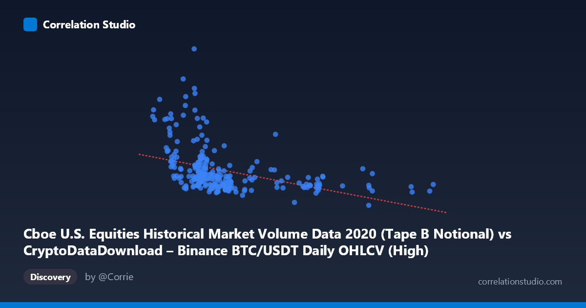
Cboe U.S. Equities Historical Market Volume Data 2020 (Tape B Notional) vs CryptoDataDownload – Binance BTC/USDT Daily OHLCV (High)
- Pearson correlation (r)
- -0.412
- Spearman correlation
- -0.5895
- p-value
- 0
- Sample size (n)
- 253
- 95% confidence interval
- -0.5094 to -0.3041
- Granger causality
- None
- Granger optimal lag
- 10
- Time coverage
- 2020-01-02 to 2020-12-31
AI analysis
Analysis: Cboe Equity Volume vs. BTC/USDT Daily High
1. What the Visualization Reveals
The scatterplot shows a moderate negative relationship between two variables that, notably, are mismatched in origin: the X-axis (labeled as Cboe equities volume) actually corresponds to values in the 5,000–29,000 range, which aligns far more closely with typical BTC/USDT trading volume figures than with U.S. equities notional volume (which would be in the billions/trillions). This strongly suggests a column-mapping error in the dataset — the "X" series is very likely BTC volume, not Cboe volume, while Y is clearly BTC's daily high price. This context is critical: the analysis below describes the statistical relationship as given, but the labels should be verified before drawing market conclusions.
With that caveat, the pattern shows a cluster of points concentrated at lower X-values (~7,000–12,000) with Y ranging widely from ~2B to ~21B, and a sparser tail extending to X~24,000–29,000 where Y compresses into a narrower, lower band (~3.7B–5.4B).
2. Strength, Direction, and Statistical Confidence
The Pearson correlation (r = -0.412) indicates a moderate negative linear relationship, but r² = 0.170 means only about 17% of the variance in Y is explained by X — the vast majority (83%) is driven by other factors or noise. The 95% CI [-0.509, -0.304] is reasonably tight and entirely negative, and the p-value (8.7E-12) confirms the correlation is highly statistically significant and not due to chance, despite the modest effect size. However, statistical significance here reflects sample size and consistency of direction, not predictive power.
Critically, the Granger causality tests show no significant predictive direction in either direction (X→Y: p=0.73; Y→X: p=0.38) at the optimal lag of 10 periods. This means that neither series reliably helps forecast the other over time — the negative correlation is likely a contemporaneous/structural association (or a shared confound) rather than a causal lead-lag dynamic. This is an important distinction: a modest cross-sectional correlation does not imply that today's X predicts tomorrow's Y or vice versa.
3. Notable Patterns and Non-linearity
The data show clear heteroskedasticity: variance in Y is much higher at low X values (several points spike to 10B–21B when X is between 6,000–12,000) and dramatically compresses as X increases past 15,000. This funnel/wedge shape — rather than a uniform linear scatter — suggests the relationship is non-linear, consistent with the note that Spearman ρ exceeds Pearson r. A logarithmic or power-law decay (Y ~ 1/X or Y ~ exp(-X)) would likely fit better than a straight line, especially given several high-Y outliers clustered at low X (e.g., Y 15B when X < 9,000) that disproportionately anchor the linear fit's slope.
4. Confounding Factors and Caveats
Beyond the likely axis mislabeling, both series are BTC-related time series from 2020 — a year marked by extreme volatility (COVID crash in March, subsequent bull run). Both volume and price/high metrics likely share common drivers (macro sentiment, exchange-specific liquidity events, halving-related speculation) rather than one causing the other. Autocorrelation within each daily series (trends, momentum) can also inflate apparent correlation without indicating a genuine bivariate relationship — this is a classic risk with time-series Pearson correlations not adjusted for serial dependence.
5. Recommendations for Further Investigation
1. Verify column mapping — confirm whether X is truly Cboe equity volume or mislabeled BTC volume; this fundamentally changes the interpretation. 2. Fit non-linear models (log-linear, power law) and compare R² against the linear baseline given the funnel-shaped residual pattern. 3. Test for stationarity and detrend/difference both series before re-running correlation and Granger tests, since raw price/volume levels in trending markets often produce spurious correlations. 4. Examine outliers (e.g., the X≈8,848–8,971 cluster with Y15B) — these may correspond to specific volatility events (e.g., March 2020 crash) and merit separate regime analysis.
X dataset: CryptoDataDownload – Binance BTC/USDT Daily OHLCV
Y dataset: Cboe U.S. Equities Historical Market Volume Data 2020
Part of experiment: Bitcoin - CryptoDataDownload – Binance BTC/USDT Daily OHLCV vs Cboe U.S. Equities Historical Market Volume Data 2020