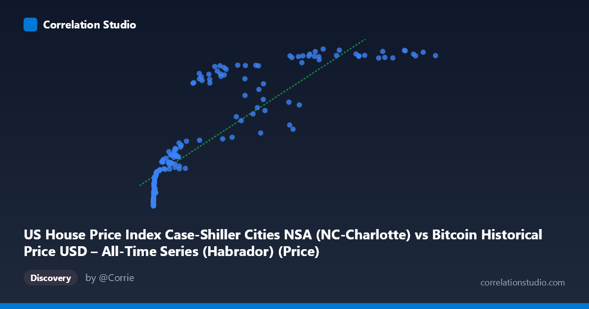
US House Price Index Case-Shiller Cities NSA (NC-Charlotte) vs Bitcoin Historical Price USD – All-Time Series (Habrador) (Price)
- Pearson correlation (r)
- 0.8553
- Spearman correlation
- 0.9686
- p-value
- 0
- Sample size (n)
- 187
- 95% confidence interval
- 0.8113 to 0.8896
- Granger causality
- None
- Granger optimal lag
- 1
AI analysis
Analysis: Bitcoin Price vs. US House Price Index (Charlotte, NC)
1. What the Visualization Reveals
The scatterplot shows a strong positive association between Bitcoin's historical USD price and the Case-Shiller Home Price Index for Charlotte, NC. However, the relationship is clearly non-linear: at low Bitcoin prices (under ~$1,000), the HPI values cluster tightly in a narrow band (108–150), while as Bitcoin prices climb into the tens/hundreds of thousands, the HPI values rise more steeply and with greater dispersion (up to 288). This produces a curved, logarithmic-like pattern rather than a straight line — consistent with the note that Spearman's ρ exceeds Pearson's r.
2. Strength, Direction, and Uncertainty
The Pearson correlation (r = 0.855) indicates a strong positive linear relationship, with r² = 0.732 meaning roughly 73% of the variance in the HPI is statistically explained by Bitcoin price (and vice versa, since correlation is symmetric). The 95% CI [0.811, 0.890] is tight and the p-value ≈ 0, indicating this correlation is highly unlikely to be due to chance in this sample. However, correlation here almost certainly reflects shared temporal trends rather than a causal economic relationship — both series have risen over the 2010–2026 window, which mechanically inflates correlation in time-series data. This is reinforced by the Granger causality tests: neither direction is significant (Bitcoin→HPI: p = 0.243; HPI→Bitcoin: p = 0.106), meaning past values of one series do not meaningfully help predict future values of the other. In other words, despite the strong contemporaneous correlation, there is no evidence of genuine predictive/causal linkage.
3. Notable Patterns and Outliers
- Compressed low-end cluster: Nearly all data points with X < $2,000 (Bitcoin's early years) sit in a tight HPI range of 108–150, reflecting Charlotte's relatively stable, slow-growing housing market pre-2017. - Fanning/divergence at high X: Once Bitcoin exceeds ~$40,000, HPI values scatter between 190 and 288 for similar X values (e.g., $56,973 → 228 vs. $58,254 → 280), suggesting the housing index's own dynamics (seasonality, 2021–2022 US housing boom) dominate independent of Bitcoin's price at that time. - Non-monotonic HPI dips: Points like (44,354 → 243) and (45,093 → 192.68) or (58,724 → 197) sitting near much higher-valued neighbors suggest genuine HPI volatility (likely reflecting the 2022 housing correction) uncorrelated with Bitcoin's contemporaneous level.
4. Confounding Factors and Caveats
The most important caveat: both series are trending, non-stationary time series over the same calendar period (2010–2026). Any two upward-trending series will show spurious correlation regardless of true causal linkage — a classic time-series pitfall. Likely shared confounders include macroeconomic conditions (near-zero interest rates 2010–2021, subsequent Fed tightening, inflation, quantitative easing) that pushed up both risk assets and real estate simultaneously. Charlotte's HPI is also a regional/local measure, while Bitcoin is a global asset, making a structural economic link implausible. The non-linear (compressed-then-fanning) shape further suggests the linear r/r² overstates the "true" strength of association; a log-transform of Bitcoin price would likely fit better and yield a different effective r².
5. Actionable Insights
- Do not treat this correlation as tradable or causal. The failed Granger tests confirm neither series leads the other in a statistically useful way. - Re-run analysis on detrended or differenced data (e.g., % monthly changes rather than levels) to test whether a genuine short-term relationship exists once shared trend is removed. - Apply a log transform to Bitcoin price before correlating, given the evident logarithmic shape, and compare r² to the linear model. - Introduce macro control variables (interest rates, CPI, M2 money supply) to test whether the observed correlation is fully mediated by common monetary conditions. - Treat this pairing primarily as an illustration of spurious correlation risk in trending time series, useful for pedagogical purposes rather than investment inference.
X dataset: Bitcoin Historical Price USD – All-Time Series (Habrador)
Y dataset: US House Price Index Case-Shiller Cities NSA
Part of experiment: Bitcoin - Bitcoin Historical Price USD – All-Time Series (Habrador) vs US House Price Index Case-Shiller Cities NSA