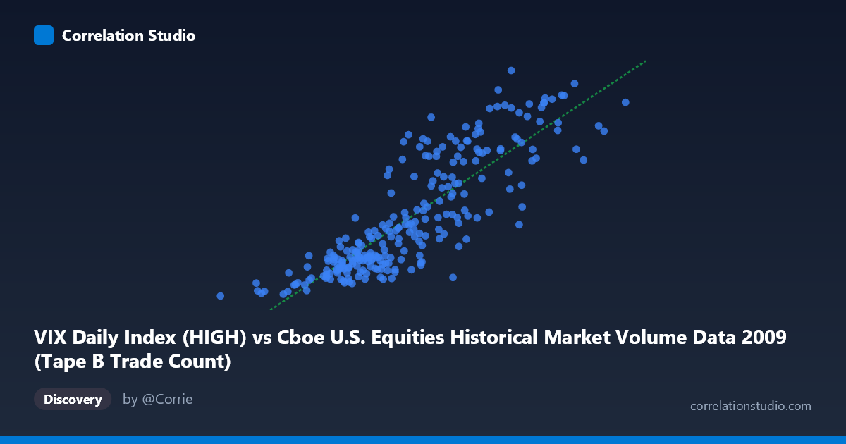
VIX Daily Index (HIGH) vs Cboe U.S. Equities Historical Market Volume Data 2009 (Tape B Trade Count)
- Pearson correlation (r)
- 0.85
- Spearman correlation
- 0.8596
- p-value
- 0
- Sample size (n)
- 252
- 95% confidence interval
- 0.8117 to 0.881
- Granger causality
- None
- Granger optimal lag
- 1
AI analysis
Scatterplot Analysis: VIX High vs. Tape B Trade Count (2009)
Relationship Overview The scatterplot reveals a clear, positive linear relationship between the VIX Daily Index High values and the Cboe U.S. Equities Tape B Trade Count throughout 2009. As the VIX High increases, Tape B trade counts rise correspondingly, following a reasonably tight upward trajectory consistent with the fitted regression line (y = 6.555×10⁻⁵x + 6.444). This aligns intuitively with market dynamics: elevated volatility environments tend to drive heightened trading activity across equity segments, including Tape B securities (primarily NYSE American and regional exchange-listed stocks). The relationship is visible across the full range of the data, from low-volatility, low-volume sessions to high-volatility, high-volume extremes.
Correlation Strength and Statistical Significance The correlation is strong and statistically robust (r = 0.85, r² = 0.7225), meaning approximately 72.3% of the variance in Tape B trade counts is explained by the VIX High level — a substantial explanatory share for financial market data. The 95% confidence interval of [0.812, 0.881] is notably narrow, reflecting the large sample size (n = 252 paired observations drawn from a population of N = 3,232), and the p-value of effectively zero confirms there is no plausible chance this association arose randomly. However, the Granger causality results are unambiguous in both directions — neither X→Y (F = 0.0017, p = 0.967) nor Y→X (F = 0.0018, p = 0.966) achieves significance at any conventional threshold. This critically means that while the two variables move together strongly in a contemporaneous sense, neither series temporally predicts the other at a one-period lag. The relationship is synchronous rather than directionally causal, suggesting both variables are likely responding simultaneously to the same underlying market conditions rather than one driving the other sequentially.
Notable Patterns, Clusters, and Outliers The data exhibits several structural features worth noting. There is a visible clustering of observations in the lower-left region (VIX High roughly 200,000–400,000; Tape B counts ~20–30), reflecting the more typical low-to-moderate volatility regime that dominated much of mid-to-late 2009 as markets recovered from the financial crisis. A second, sparser upper-right cluster (VIX High above 550,000; counts above 40) corresponds to high-stress trading sessions, likely concentrated in early 2009 during peak crisis volatility. A few points — notably near the extremes (e.g., VIX ~766,764 with count ~52, and the minimum at ~81,703 with count ~19.67) — anchor the regression line but may exert disproportionate leverage. The spread around the regression line widens somewhat at higher VIX values, suggesting mild heteroscedasticity, and there are isolated mid-range observations (e.g., ~591,944 VIX but only ~34.56 count) that deviate notably from the trend, hinting at occasional decoupling.
Confounding Factors and Interpretive Caveats Several important caveats apply. First, 2009 was a structurally unusual year — spanning the tail of the worst financial crisis since the Great Depression and the subsequent recovery — meaning the variance-volatility relationship captured here may not generalize to normal market regimes. The extreme range of VIX values (81,703 to 766,764) compresses what in calmer years would be a much narrower distribution. Second, Tape B trade counts are influenced by factors beyond volatility, including exchange fee structures, algorithmic routing decisions, order fragmentation patterns, and the secular growth of electronic trading during this period — all of which could independently correlate with both variables. Third, the absence of Granger causality at lag 1 may partly reflect that the relevant predictive lag is intraday rather than daily, a limitation of the daily frequency data used here. Finally, the linear regression assumption deserves scrutiny given the visual suggestion of heteroscedasticity and possible nonlinearity at the tails.
Actionable Insights and Further Investigation Practitioners and researchers should consider several follow-up analyses. First, testing for non-linear functional forms (e.g., log-log or polynomial regression) could improve fit, particularly at VIX extremes, and may reveal threshold effects where Tape B volume accelerates disproportionately above certain volatility levels. Second, decomposing the analysis by market regime (pre/post March 2009 market bottom) would clarify whether the relationship is stable across the year or driven primarily by the crisis period. Third, given the failed Granger test, investigating intraday data or introducing contemporaneous controls (e.g., overall market volume, S&P 500 returns, bid-ask spreads) could better isolate whether VIX and Tape B volume are jointly determined by a common latent factor such as investor fear or institutional rebalancing flows. Finally, extending this analysis to multiple years would test whether 2009's crisis dynamics produced an artificially inflated correlation that diminishes in calmer periods.
X dataset: Cboe U.S. Equities Historical Market Volume Data 2009
Y dataset: VIX Daily Index
Part of experiment: Daily - Cboe U.S. Equities Historical Market Volume Data 2009 vs VIX Daily Index