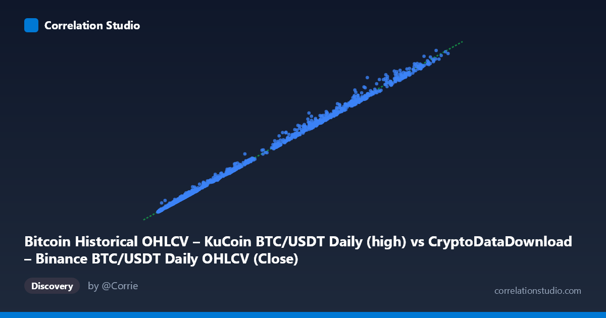
Bitcoin Historical OHLCV – KuCoin BTC/USDT Daily (high) vs CryptoDataDownload – Binance BTC/USDT Daily OHLCV (Close)

Pearson correlation (r): 0.9992
Spearman correlation: 0.9986
p-value: 0
Sample size (n): 1861
95% confidence interval: 0.9991 to 0.9992
Granger causality: None
Granger optimal lag: 10
Time coverage: 2017-10-19 to 2022-11-29

AI analysis

Analysis: BTC/USDT Daily High (Binance) vs. Close (KuCoin)

1. Relationship Overview

The scatterplot depicts an almost perfectly linear relationship between Binance's daily high price and KuCoin's daily close price for BTC/USDT, spanning October 2017 through November 2022. Points hug a tight diagonal band across the entire price range (~$3,200 to ~$69,000), with no visible curvature, fanning, or regime breaks. This is expected: both series track the same underlying asset (Bitcoin) priced in the same quote currency (USDT) on two highly liquid, arbitrage-linked exchanges.

2. Strength, Direction, and Statistical Meaning

The correlation is essentially maximal: r = 0.9992, r² = 0.9983, meaning 99.83% of the variance in KuCoin's close price is explained by Binance's daily high — leaving less than 0.2% attributable to noise, exchange-specific microstructure, or timing differences. The 95% CI [0.9991, 0.9992] is extremely narrow given the large sample (n=1,861), and the p-value of 0 (effectively <10⁻³⁰⁰) confirms this is not a chance finding. The regression slope (1.027) close to 1 and small intercept ($33.44) indicate the two series are nearly interchangeable in scale, with KuCoin's close running marginally above Binance's high on average — plausible since "high" is an intraday ceiling while "close" is a separate daily snapshot that can occasionally exceed it.

Importantly, the Granger causality test found no significant predictive direction in either direction (X→Y: p=0.36; Y→X: p=0.33) at the optimal 10-lag structure. This means neither series' historical values help forecast the other's future values beyond what each series' own history provides. This is the crucial nuance: high contemporaneous correlation does not imply lead-lag predictability. Both series are likely driven by a common latent factor (the "true" global BTC price) rather than one exchange causally driving the other with a temporal lag.

3. Patterns, Clusters, and Outliers

The data naturally clusters into groups reflecting Bitcoin's historical price regimes: a dense cluster below $10,000 (2018–2019 bear market and consolidation), a mid-range cluster around $19,000–$30,000 (2019 rally / 2021 correction), and sparser points above $40,000–$69,000 (2020–2021 bull run peak). Because both stdevs (~17,000–17,400) and ranges are similar, the point cloud is roughly homoscedastic in log-space but shows increasing absolute dispersion at higher price levels — a few sample rows (e.g., 29,103.94 vs. 32,256.00 close) show larger absolute deviations, consistent with higher volatility (in dollar terms) during high-price/high-volatility periods rather than true divergence. No structural outliers or discontinuities are evident from the samples shown.

4. Confounding Factors and Caveats

Several caveats apply: (a) this is not two independent phenomena but the same asset measured on two exchanges with arbitrage keeping prices tightly bound — the "correlation" mostly reflects market efficiency and cross-exchange arbitrage, not two distinct causal series; (b) comparing a "high" to a "close" mixes different intraday statistics, so residual differences partly reflect intraday range/volatility rather than exchange divergence; (c) daily aggregation masks any short-term (intra-day or few-hour) lead-lag relationships that a Granger test on daily data with 10 lags may not detect; (d) both series share non-stationarity (trending price data), which inflates correlation coefficients — this "spurious regression" risk should be checked via cointegration tests rather than relying on r² alone.

5. Suggestions for Further Investigation

- Test cointegration (e.g., Engle-Granger) rather than simple correlation, given the non-stationary price trends. - Re-run Granger causality on returns (log differences) or on higher-frequency (hourly/minute) data, where genuine lead-lag microstructure effects (e.g., price discovery leadership between Binance and KuCoin) are more likely to emerge. - Examine the residuals (Y − regression prediction) over time to detect any periods of exchange-specific stress, outages, or liquidity gaps (e.g., flash crashes) where divergence temporarily spikes. - Compare against Binance's own close (rather than high) to isolate whether the price differences stem from the exchange or the OHLC field choice.

X dataset: CryptoDataDownload – Binance BTC/USDT Daily OHLCV

Y dataset: Bitcoin Historical OHLCV – KuCoin BTC/USDT Daily

Part of experiment: Bitcoin - CryptoDataDownload – Binance BTC/USDT Daily OHLCV vs Bitcoin Historical OHLCV – KuCoin BTC/USDT Daily