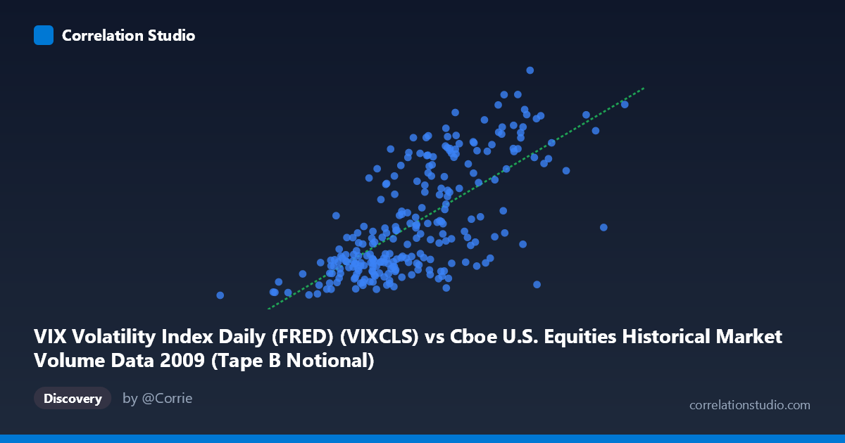
VIX Volatility Index Daily (FRED) (VIXCLS) vs Cboe U.S. Equities Historical Market Volume Data 2009 (Tape B Notional)
- Pearson correlation (r)
- 0.693
- Spearman correlation
- 0.6837
- p-value
- 0
- Sample size (n)
- 252
- 95% confidence interval
- 0.6228 to 0.7522
- Granger causality
- None
- Granger optimal lag
- 1
AI analysis
Analysis: VIX Volatility Index vs. Cboe Tape B Notional Volume (2009)
Relationship Overview
The scatterplot reveals a moderate-to-strong positive relationship between the CBOE Volatility Index (VIX) and Tape B notional trading volume on U.S. equity exchanges throughout 2009. As VIX values rise — indicating greater market fear and implied volatility — Tape B notional volume tends to increase correspondingly. This is an intuitively sensible finding: periods of elevated market stress characteristically trigger heightened trading activity as investors reposition, hedge, or liquidate holdings. The linear regression equation (y = 4.80×10⁻⁹x + 6.14) confirms a positive slope, and the visual scatter broadly supports this upward trend, though with considerable dispersion around the regression line.
Correlation Strength and Statistical Significance
The Pearson correlation of r = 0.693 indicates a meaningful positive association, with r² = 0.4803 meaning that approximately 48% of the variance in VIX is explained by Tape B notional volume (or vice versa) — a substantial but incomplete explanatory relationship, leaving roughly 52% of variance attributable to other factors. The 95% confidence interval of [0.623, 0.752] is relatively narrow given the sample size of n = 252, and the p-value of ~0 confirms the correlation is highly statistically significant and extremely unlikely to be a chance artifact. However, the Granger causality tests tell a more cautious story: neither direction (X→Y: F = 0.043, p = 0.837; Y→X: F = 0.360, p = 0.549) achieves significance, meaning that neither variable reliably predicts the other temporally at a 1-period lag. This is a critical nuance — the variables move together contemporaneously, but neither leads the other in a predictive sense.
Notable Patterns, Clusters, and Outliers
The scatterplot exhibits several structural features worth noting. There appears to be a distinct clustering at lower VIX values (roughly 20–30) paired with a wide spread of notional volumes, suggesting that in calmer market regimes the volume relationship is less predictable. At higher VIX levels (40–55), points tend to congregate at elevated notional volumes, reflecting the crisis-driven trading environment of early-to-mid 2009 — a residual of the 2008 financial crisis spillover. Several outlier points are visible at high VIX readings with notional volume exceeding 7–9 billion, likely corresponding to specific volatility spikes (e.g., March 2009 market lows). Conversely, some moderate-VIX observations show surprisingly low notional values, hinting at non-linearity or threshold effects in the relationship that a simple linear model may not fully capture.
Confounding Factors and Caveats
Several important caveats limit straightforward causal interpretation. 2009 is an extraordinary year — spanning the tail end of the global financial crisis through the subsequent recovery — meaning results may not generalize to normal market conditions. Tape B specifically covers NYSE American (AMEX) and regional exchange-listed securities, a subset of total market activity, which may behave differently from the broader market that VIX reflects (which is anchored to S&P 500 options). Temporal autocorrelation in both financial time series (VIX persistence, volume clustering) can inflate perceived correlations. Additionally, algorithmic and high-frequency trading activity in 2009 was accelerating rapidly, potentially driving notional volume independent of sentiment. The Granger causality null result also warns against assuming the VIX "drives" volume decisions in any mechanistic, time-lagged way.
Actionable Insights and Further Investigation
Practitioners and researchers should consider several follow-up directions. First, segmenting the data into crisis (Q1 2009) vs. recovery (Q3–Q4 2009) regimes would likely reveal whether the correlation is driven predominantly by the high-volatility period or persists across market conditions. Second, testing non-linear models (e.g., quadratic, log-log, or piecewise regression) could better capture the apparent threshold behavior at extreme VIX levels. Third, extending the analysis to Tape A and Tape C notional volumes would clarify whether this relationship is specific to smaller-cap exchange listings or is a market-wide phenomenon. Finally, incorporating intraday data or shorter lag structures in Granger tests might uncover predictive relationships missed at the daily lag examined here, since volatility-volume dynamics in modern markets can operate on minute-level timescales.
X dataset: Cboe U.S. Equities Historical Market Volume Data 2009
Y dataset: VIX Volatility Index Daily (FRED)
Part of experiment: Daily - Cboe U.S. Equities Historical Market Volume Data 2009 vs VIX Volatility Index Daily (FRED)