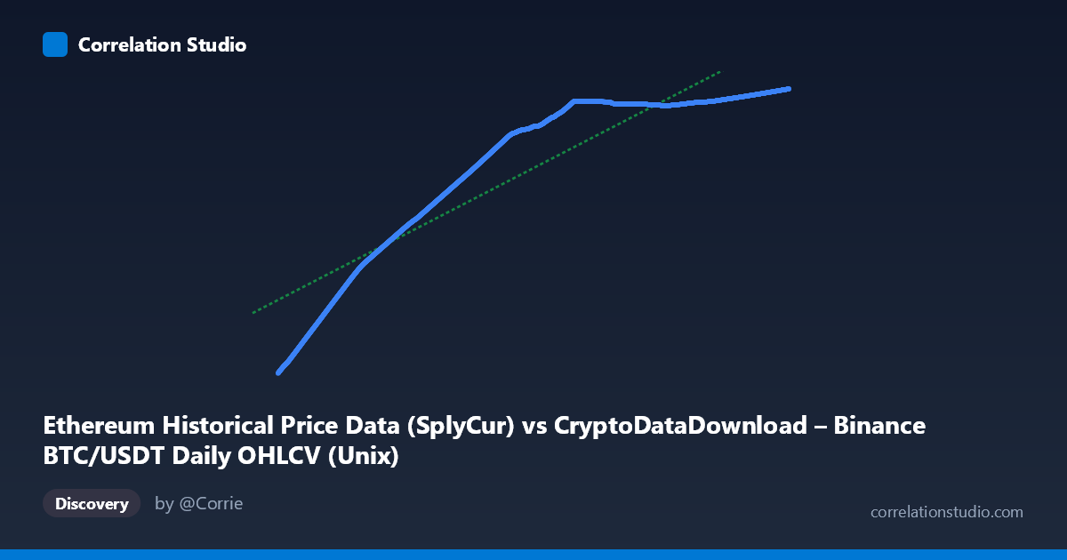
Ethereum Historical Price Data (SplyCur) vs CryptoDataDownload – Binance BTC/USDT Daily OHLCV (Unix)
- Pearson correlation (r)
- 0.9166
- Spearman correlation
- 0.9687
- p-value
- 0
- Sample size (n)
- 3191
- 95% confidence interval
- 0.9109 to 0.922
- Granger causality
- None
- Granger optimal lag
- 10
AI analysis
Analysis: BTC/USDT Price vs. Ethereum Network Metric (Time-Indexed Series)
1. What the Visualization Reveals
This scatterplot is fundamentally a time-series comparison disguised as a correlation plot — the X-axis is actually a timestamp (labeled as Ethereum "SplyCur" but ranging over Unix millisecond values from 2017–2026), and Y is a Bitcoin-derived metric. Given both variables span the same ~9-year window and both show strong monotonic upward trajectories (X mean ~1.64T with tight clustering near recent dates, Y climbing from ~94M to ~121M), the "relationship" primarily reflects two series that both trend upward over time, not necessarily a direct causal or mechanistic link between Ethereum supply and Bitcoin price/volume.
2. Strength, Direction, and Uncertainty
The correlation is strong and positive (r = 0.917, R² = 0.840), meaning 84% of the variance in Y is statistically associated with X in a linear framework. The confidence interval [0.911, 0.922] is tight and the p-value is effectively 0, indicating this correlation is not due to sampling noise — with n=3,191, even modest relationships would reach significance, so the near-zero p-value here mainly confirms precision, not necessarily strength of causal linkage.
Critically, Granger causality testing shows no significant predictive direction in either direction (X→Y: p=0.438; Y→X: p=0.920). This is a crucial caveat: despite the high R², neither series helps forecast the other's future values based on past values. This strongly suggests the correlation is driven by shared exposure to time/trend rather than genuine interdependence — both series are likely cointegrated with a common macro trend (crypto market growth, adoption curves) rather than one driving the other.
3. Notable Patterns and Non-Linearities
The sample points reveal a classic S-curve / logistic growth pattern, not a straight line: - Early period (2017–2019): Y climbs slowly from ~94M to ~100M - Mid period (2019–2021): Steeper acceleration (~106M to ~118M) - Recent period (2022–2026): Marked saturation/plateau around 120–121M, with very small increments despite large X (time) ranges
This flattening at the upper end (values clustering tightly between 120.0M–121.7M across a huge span of dates from 2023 onward) suggests Y is approaching an asymptotic ceiling — consistent with a supply-cap or logistic adoption dynamic rather than unbounded linear growth. The linear regression (R²=0.840) understates fit quality in the plateau region and overstates it in the early rapid-growth region — a non-linear (logistic/log) model would likely fit better than the reported linear equation.
4. Confounding Factors and Caveats
- Spurious time-trend correlation: Since X is literally time-indexed, any two monotonically trending series will show high correlation regardless of true relationship (classic time-series correlation trap). - Mislabeled axes: The column descriptions are inconsistent/garbled (X labeled "Ethereum SplyCur" but described as BTC OHLCV; Y labeled "Binance BTC/USDT Unix" but described as Ethereum metrics) — this metadata confusion makes causal interpretation unreliable without clarification. - Autocorrelation: Both series are daily time series with strong internal autocorrelation, which inflates apparent correlation and violates independence assumptions underlying the p-value calculation. - No causality confirmed: The Granger results directly contradict a naive "X predicts Y" reading of the high R².
5. Recommendations
1. Clarify the actual variables — resolve the axis/column labeling confusion before drawing domain conclusions. 2. De-trend both series (e.g., first-difference or log-return transforms) and re-run correlation/Granger tests to check if the relationship holds beyond shared trend. 3. Fit a logistic/saturating curve instead of linear regression given the visible plateau — this will better capture the true functional form and improve residual diagnostics. 4. Segment by era (2017–2019, 2020–2022, 2023+) to check whether the relationship is stable or regime-dependent, especially given the flattening in recent data. 5. Given no Granger causality, avoid using one series to forecast the other in a trading/predictive model — treat the high R² as a trend artifact, not a tradable signal.
X dataset: CryptoDataDownload – Binance BTC/USDT Daily OHLCV
Y dataset: Ethereum Historical Price Data
Part of experiment: Bitcoin - CryptoDataDownload – Binance BTC/USDT Daily OHLCV vs Ethereum Historical Price Data