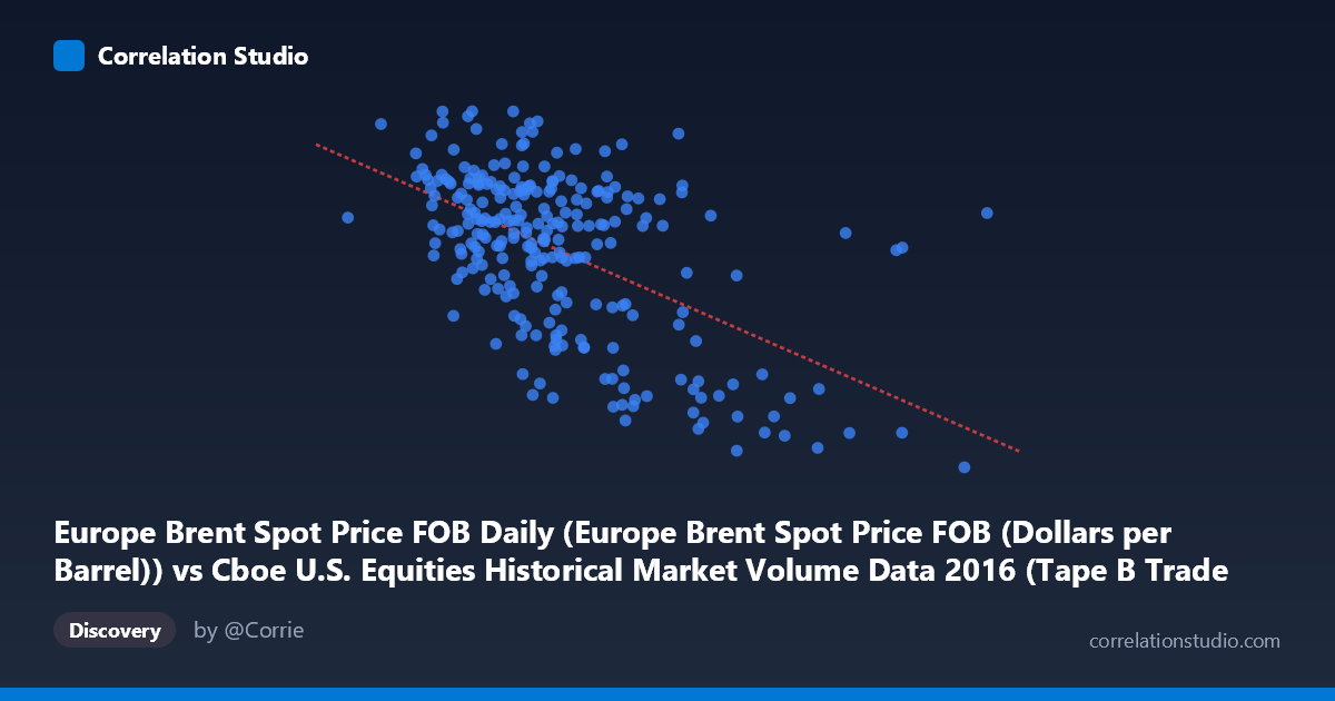
Europe Brent Spot Price FOB Daily (Europe Brent Spot Price FOB (Dollars per Barrel)) vs Cboe U.S. Equities Historical Market Volume Data 2016 (Tape B Trade Count)
- Pearson correlation (r)
- -0.5472
- Spearman correlation
- -0.4797
- p-value
- 0
- Sample size (n)
- 251
- 95% confidence interval
- -0.6285 to -0.4542
- Granger causality
- None
- Granger optimal lag
- 1
AI analysis
Analysis: Europe Brent Spot Price vs. Cboe Tape B Trade Count (2016)
Relationship Overview The scatterplot reveals a negative relationship between Europe Brent Spot Price (X-axis, in dollars per barrel) and Cboe Tape B Trade Count (Y-axis), meaning that as oil prices were higher, equity trade counts on Tape B tended to be lower, and vice versa. The linear regression equation (y = -3.856×10⁻⁵x + 55.99) confirms this inverse slope. Visually, the data show a moderately dispersed cloud with a discernible downward trend, though substantial scatter around the regression line is evident, particularly in the mid-range of oil prices (~$250,000–$350,000 range on the X-axis, which appears to represent a scaled or transformed price metric).
Correlation Strength and Statistical Significance The Pearson correlation of r = -0.547 indicates a moderate negative association. The R² value of 0.30 means that approximately 30% of the variance in Tape B trade counts is explained by Brent spot prices — meaningful, but leaving 70% of variance unexplained by this relationship alone. The 95% confidence interval of [-0.629, -0.454] is entirely negative and reasonably tight, confirming the direction and moderate magnitude of the association with good reliability. The p-value of effectively zero (given N = 3,622) confirms this is highly statistically significant and not a chance finding. However, the Granger causality tests reveal no significant temporal predictive direction in either direction (X→Y: F = 0.387, p = 0.535; Y→X: F = 0.936, p = 0.334), meaning that despite the contemporaneous correlation, past Brent prices do not reliably predict future Tape B trade counts, and vice versa. This is a critical nuance: the two variables move together, but neither demonstrably leads the other.
Notable Patterns, Clusters, and Outliers Several features stand out in the data. The bulk of observations cluster in the $200,000–$380,000 X-range with Y values between roughly 40–53, forming a relatively dense central cloud. There is a notable lower-right cluster of points with high X values (above $400,000–$550,000) and markedly low Y values (26–34), including an extreme point near (693,228, 26.01) and another near (558,190, 27.59) — these high-price, low-trade-count observations appear to be influential outliers that likely strengthen the negative correlation considerably. There also appear to be a few high-Y outliers at lower X values (e.g., ~202,782, 53.01), suggesting that low oil price periods occasionally coincided with unusually high trading activity. The relationship appears somewhat non-linear, with a steep drop-off at extreme X values rather than a smooth linear decline throughout.
Confounding Factors and Caveats Several important caveats apply. First, both variables are time series from 2016, meaning shared temporal trends, seasonality, or common macro shocks (e.g., OPEC decisions, U.S. election volatility, commodity super-cycle dynamics) could be driving a spurious correlation rather than any direct mechanism. The absence of Granger causality strongly supports this concern. Second, Tape B trade count reflects equities exchange activity for a specific tape segment, which is influenced by countless factors — volatility regimes, algorithmic trading activity, market structure changes — largely unrelated to oil prices. Third, the X-axis scale (values in the hundreds of thousands for what should be ~$30–$55/barrel oil prices) suggests a data alignment or scaling issue that warrants verification; the datasets may not be perfectly paired or the X variable may represent a composite or transformed metric. Finally, N = 3,622 vs. n = 251 implies the sample is a fraction of the full dataset, and sampling methodology could affect representativeness.
Actionable Insights and Further Investigation Given the moderate correlation but absent Granger causality, the association likely reflects co-movement driven by common macro factors rather than a direct or predictive relationship. Investigators should: (1) verify the data alignment and unit scaling on the X-axis, as the values appear inconsistent with raw Brent prices; (2) control for time trends and seasonality using regression with date-based controls or differenced series to isolate genuine co-movement; (3) test for non-linear specifications (e.g., polynomial or spline regression), as the outlier cluster suggests the linear model may be too simplistic; (4) examine the high-leverage outliers individually — the extreme high-X, low-Y points may correspond to specific macro events (e.g., oil price shocks) that disproportionately influence the correlation; and (5) explore mediating variables such as overall market volatility (VIX), broader equity market volume, or sector-specific trading flows to better explain the remaining 70% of variance.
X dataset: Cboe U.S. Equities Historical Market Volume Data 2016
Y dataset: Europe Brent Spot Price FOB Daily
Part of experiment: Daily - Cboe U.S. Equities Historical Market Volume Data 2016 vs Europe Brent Spot Price FOB Daily