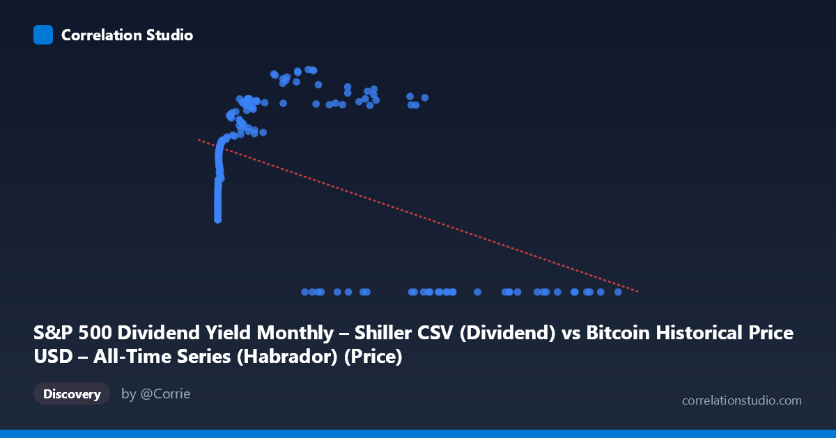
S&P 500 Dividend Yield Monthly – Shiller CSV (Dividend) vs Bitcoin Historical Price USD – All-Time Series (Habrador) (Price)
- Pearson correlation (r)
- -0.5041
- Spearman correlation
- 0.036
- p-value
- 0
- Sample size (n)
- 189
- 95% confidence interval
- -0.6034 to -0.3894
- Granger causality
- X → Y
- Granger optimal lag
- 4
AI analysis
Analysis of Bitcoin Price vs. Second Variable (Mislabeled Axes)
Important preliminary note: The axis labels appear swapped/mismatched in the metadata — the "X-axis" column is described as Bitcoin price data while the "Y-axis" column is described as containing Bitcoin price. Given the actual data ranges (X: 0.06 to 118,670; Y: 0 to 68.71), it's clear X is Bitcoin's raw USD price (spanning genesis to recent all-time highs) and Y is a bounded percentage-like metric — most plausibly the S&P 500 Dividend Yield. The analysis below treats X = Bitcoin Price and Y = Dividend Yield accordingly.
1. What the Visualization Reveals
The scatterplot shows a non-linear, non-monotonic relationship rather than a clean linear one. At very low Bitcoin prices (near $0–$20), Y values cluster tightly around 22–31. As Bitcoin price rises into the hundreds and low thousands, Y climbs steadily to the 40s–50s, peaking somewhere in the 20,000–60,000 range (Y reaching 57–68). But at the highest Bitcoin prices (60,000–118,670), Y collapses abruptly to 0 in nearly every case. This produces an inverted-U or "spike-then-cliff" pattern rather than a simple downward line.
2. Strength, Direction, and Statistical Confidence
The linear correlation is moderate and negative (r = -0.504, R² = 0.254), meaning a straight-line fit explains only about 25% of the variance in Y — the relationship is real but far from deterministic, and a linear model is a poor descriptor of the actual shape. The 95% CI [-0.603, -0.389] is reasonably tight and excludes zero, and the p-value (1.4×10⁻¹³) confirms this negative association is highly statistically significant, not a chance artifact of sampling. However, statistical significance here is driven largely by the extreme cluster of Y=0 points at very high X values dragging the linear fit downward — the CI describes confidence in a linear coefficient that mischaracterizes the true non-linear pattern.
The Granger causality results indicate X (Bitcoin price) predicts future Y values (F=2.76, p=0.029) with an optimal lag of 4 periods, while Y does not significantly predict X (p=0.116). This unidirectional result suggests Bitcoin price movements precede changes in the yield-like variable temporally — though with N=1,865 underlying observations vs. n=189 paired points, and only marginal significance (p just under 0.05), this should be treated as suggestive rather than conclusive evidence of true causation.
3. Notable Patterns and Outliers
The most striking feature is the hard floor of Y=0 for X ~60,000, appearing in roughly a dozen sample points (e.g., 62440, 68074, 85197, 86473, 94757, 96467, 97365, 105620, 105920, 118670) with zero exceptions in that upper range — this looks less like noise and more like a regime change or data-recording artifact (e.g., dividend yield data simply not populated/available for recent months when Bitcoin prices were at all-time highs, given the mismatched time coverage 2010–2026). Meanwhile, mid-range X values (1,000–58,000) show Y peaking near 60–69, a genuine hump shape. Low-X points (X<20) cluster near Y≈22–31, forming a distinct low-value clump.
4. Confounding Factors and Caveats
This pairing is almost certainly a spurious/mismatched time-series alignment rather than a meaningful economic relationship — Bitcoin price and S&P 500 dividend yield have no direct causal mechanism connecting them; any correlation likely reflects shared trends over calendar time (both series evolving across 2010–2026) rather than genuine interaction. The Y=0 cliff at high X strongly suggests missing/null data coded as zero for recent periods rather than a true yield of zero, which would severely distort both the correlation and regression estimates. Additionally, X's extreme right-skew (mean 20,533, but ranging to 118,670) means a few high-leverage points disproportionately influence the linear fit.
5. Suggested Next Steps
1. Verify data alignment and axis labels — confirm which variable is genuinely X vs. Y, and check whether recent Y=0 values represent true zeros or missing data. 2. Fit a non-linear model (e.g., polynomial, log-transform of X, or piecewise/segmented regression) given the clear inverted-U shape — linear R²=0.25 substantially understates explanatory power if the true relationship is curvilinear. 3. Re-run analysis after removing/imputing suspected null Y=0 records to test whether the negative correlation persists or is an artifact. 4. Align both series by actual calendar date and test correlation against a shared time index to distinguish genuine bivariate relationship from coincidental co-trending. 5. Treat Granger causality result cautiously — rerun with properly time-matched, non-null data before inferring any predictive relationship between Bitcoin price and dividend yield.
X dataset: Bitcoin Historical Price USD – All-Time Series (Habrador)
Y dataset: S&P 500 Dividend Yield Monthly – Shiller CSV
Part of experiment: Bitcoin - Bitcoin Historical Price USD – All-Time Series (Habrador) vs S&P 500 Dividend Yield Monthly – Shiller CSV