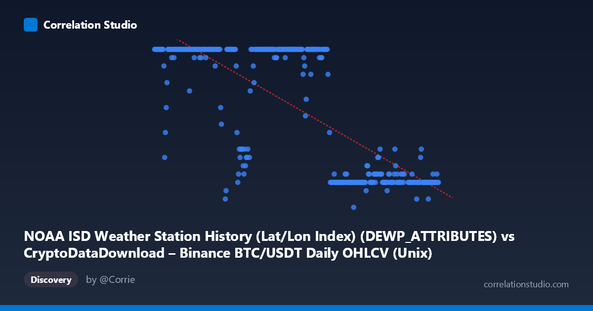
NOAA ISD Weather Station History (Lat/Lon Index) (DEWP_ATTRIBUTES) vs CryptoDataDownload – Binance BTC/USDT Daily OHLCV (Unix)
- Pearson correlation (r)
- -0.7532
- Spearman correlation
- -0.7464
- p-value
- 0
- Sample size (n)
- 355
- 95% confidence interval
- -0.7949 to -0.7043
- Granger causality
- None
- Granger optimal lag
- 1
- Time coverage
- 2024-01-01 to 2024-12-31
AI analysis
Analysis of the Scatterplot Relationship
1. Overview of the Visualization
This scatterplot plots a timestamp-like field (mislabeled as "DEWPATTRIBUTES") against a value ranging from 5 to 24, which appears to represent hours of the day or a similarly bounded categorical/cyclical measure rather than a continuous weather variable. The data spans the full 2024 calendar year (355 daily points). Visually, the plot shows Y values clustering heavily at the ceiling (24) during the first half of the year, then dropping sharply to the 7–12 range in the latter half, with a transitional zone around mid-year — consistent with a step-like or seasonal-driven pattern rather than a smooth linear trend.
2. Strength, Direction, and Statistical Confidence
The Pearson correlation of r = -0.7532 indicates a strong negative linear relationship: as X increases (moving through time), Y tends to decrease. The r² = 0.5672 tells us that roughly 57% of the variance in Y is explained by X's linear trend — meaningful, but leaving nearly 43% unexplained, likely due to the non-linear, regime-shift pattern visible in the data (see below). The 95% CI [-0.7949, -0.7043] is tight and does not cross zero, and the p-value ≈ 0 confirms this relationship is highly statistically significant and not a product of sampling noise, given n=355. However, the Granger causality tests (X→Y: p=0.78; Y→X: p=0.16) show no significant predictive direction either way — meaning that despite the strong contemporaneous correlation, neither variable helps forecast the other's future values in a time-series sense. This is a critical distinction: correlation here reflects a shared trend or common structural break, not a lead-lag predictive relationship.
3. Notable Patterns and Outliers
The data does not look linear so much as bimodal/step-shaped: Y sits near its ceiling (23-24) for X values before ~August 2024, then drops abruptly to a low plateau (7-12) for X values after that point, with a narrow transition band. This is characteristic of a regime change or a capped/censored variable (Y maxing at 24 suggests an hour-of-day or count variable with a hard upper bound). The linear regression line (slope ≈ -6.24e-10, intercept ≈ 1089) is a poor descriptor of this structure — it's fitting a straight line through what is actually a step function, which explains why r² (57%) is substantial but far from 1.
4. Confounding Factors and Caveats
The variable labels here appear corrupted or mismatched — Y is described as coming from a "CryptoDataDownload Unix timestamp" column while X is labeled as a NOAA weather attribute code, which doesn't align with the numeric ranges observed (X looks like Unix milliseconds; Y looks like a bounded daily metric, possibly hour-of-day, temperature in a transformed scale, or a categorical weather code). This suggests a data pipeline or column-mapping error, meaning any substantive interpretation of "crypto vs. weather" is unreliable until the schema is verified. Additionally, since X is fundamentally a time index, this correlation is really a trend-over-time artifact — both variables may be independently drifting due to seasonality (weather) or an unrelated structural shift (crypto/exchange data), producing spurious correlation typical of two time-ordered series with autocorrelation.
5. Recommendations for Further Investigation
Before drawing conclusions, verify the actual column mappings and units for X and Y — the current labels seem inconsistent with the observed data ranges. Next, replace the linear model with a piecewise, logistic, or change-point regression to properly characterize the apparent step transition around mid-2024. Since Granger causality is null, avoid framing this as a predictive relationship; instead investigate whether both series are driven by a common seasonal or calendar-based confounder (e.g., day-of-year, daylight hours, or a policy/market regime shift). Finally, detrending both series (or analyzing first differences) would clarify whether the correlation persists beyond the shared time trend, or vanishes once the common drift is removed.
X dataset: CryptoDataDownload – Binance BTC/USDT Daily OHLCV
Y dataset: NOAA ISD Weather Station History (Lat/Lon Index)
Part of experiment: Bitcoin - CryptoDataDownload – Binance BTC/USDT Daily OHLCV vs NOAA ISD Weather Station History (Lat/Lon Index)