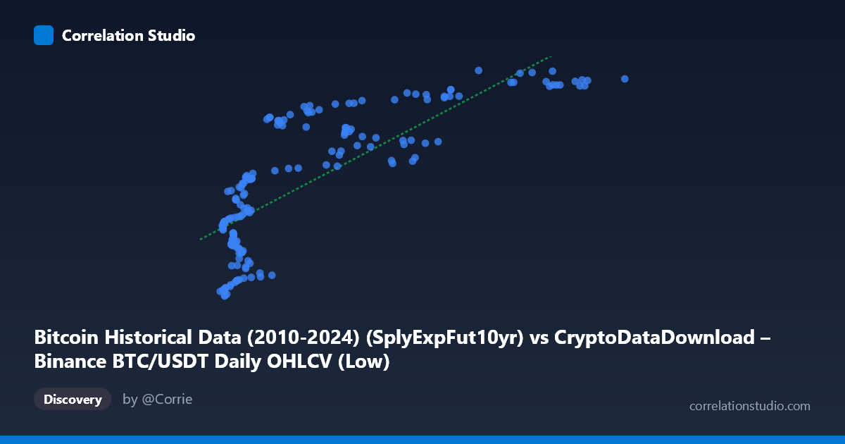
Bitcoin Historical Data (2010-2024) (SplyExpFut10yr) vs CryptoDataDownload – Binance BTC/USDT Daily OHLCV (Low)
- Pearson correlation (r)
- 0.8018
- Spearman correlation
- 0.833
- p-value
- 0
- Sample size (n)
- 180
- 95% confidence interval
- 0.7426 to 0.8486
- Granger causality
- None
- Granger optimal lag
- 10
AI analysis
Analysis of Bitcoin Price/Supply-Metric Correlation
1. What the Visualization Reveals
The scatterplot shows a clear positive, non-linear relationship between the two variables. Rather than a straight-line pattern, the data traces a curve reminiscent of a logarithmic or saturating growth function: Y rises steeply as X increases from ~2,800 to ~20,000, then the rate of increase flattens considerably as X continues to grow toward 115,000. This is visually consistent with an asset-price relationship where Y (a low/price metric) responds sharply at low X values but plateaus near an upper bound (~20.7–20.8 million) at higher X values.
2. Strength, Direction, and Statistical Confidence
The Pearson correlation of r = 0.80 indicates a strong positive linear association, but the r² = 0.643 tells the more important story: only about 64% of the variance in Y is explained by X in a linear framework — meaning over a third of the variability is left unexplained, likely due to the visible curvature (a linear model is a mis-specification here). The 95% CI [0.743, 0.849] is reasonably tight and does not cross zero, and the p-value ≈ 0 confirms this correlation is highly unlikely to be due to chance in this sample. However, correlation strength should not be conflated with causation or predictive power over time: the Granger causality tests show no significant predictive direction in either direction (X→Y: p=0.445; Y→X: p=0.682) at the optimal lag of 10 periods. This means that despite being strongly correlated in level/cross-sectional terms, past values of one series do not help forecast future values of the other — the relationship may be driven by a shared underlying trend (e.g., both being transformations of the same BTC price series) rather than one causally leading the other.
3. Notable Patterns and Features
The most striking feature is the elbow/knee shape near X ≈ 15,000–25,000, where Y transitions from a steep climb to a much flatter, near-asymptotic regime. Above X ≈ 60,000, Y values compress into a narrow band (20,750,000–20,830,000), suggesting a ceiling effect or saturation. There's no obvious clustering by distinct subgroups, but the data appears denser at low-X values, indicating BTC spent more sample-days in lower-price regimes historically. No dramatic outliers are apparent, though the point at (74,604, 20,828,425) marks the sample maximum for Y.
4. Confounding Factors and Caveats
A major caveat: both variables are derived from the same underlying Binance BTC/USDT OHLCV dataset — X is a supply-expectation-futures-linked column and Y is the "Low" price. Since both are mathematically or economically entangled with Bitcoin's price trajectory, high correlation is almost tautological rather than revealing an independent relationship. Additionally, this is time-series data (2017–2026), so autocorrelation and shared trending (both series rising over the BTC bull market) can inflate r without implying meaningful joint dynamics — classic "spurious regression" risk. The non-stationarity of price data undermines the validity of a simple Pearson r/linear R² framework.
5. Suggestions for Further Investigation
Given the curvature, a log-linear or logistic transformation of X would likely fit far better than the current linear model (y = 5.16x + 2.04×10⁷, R²=0.643) — try log(X) or a saturating function to improve fit and better justify r². Since Granger causality is absent, consider testing cointegration (e.g., Engle-Granger or Johansen test) to see if these series share a long-run equilibrium relationship despite lacking short-term predictive causality. Finally, given both columns trace back to the same exchange/price data, clarify the exact definitions of "SplyExpFut10yr" and "Low" to rule out definitional overlap before treating this as two independent signals.
X dataset: CryptoDataDownload – Binance BTC/USDT Daily OHLCV
Y dataset: Bitcoin Historical Data (2010-2024)
Part of experiment: Bitcoin - CryptoDataDownload – Binance BTC/USDT Daily OHLCV vs Bitcoin Historical Data (2010-2024)