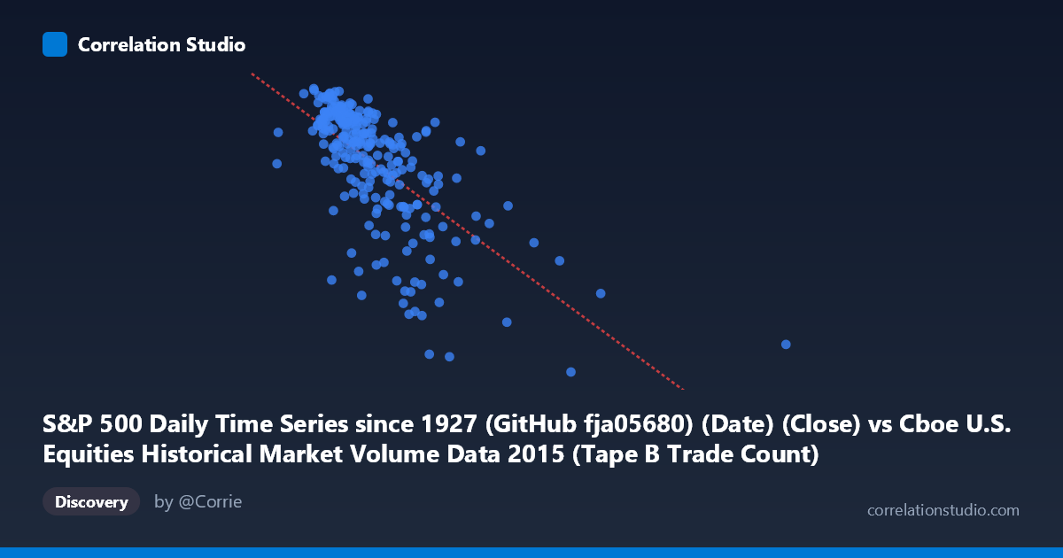
S&P 500 Daily Time Series since 1927 (GitHub fja05680) (Date) (Close) vs Cboe U.S. Equities Historical Market Volume Data 2015 (Tape B Trade Count)

Pearson correlation (r): -0.6663
Spearman correlation: -0.7066
p-value: 0
Sample size (n): 252
95% confidence interval: -0.7298 to -0.5914
Granger causality: None
Granger optimal lag: 1

AI analysis

Analysis: S&P 500 Close Price vs. Cboe Tape B Trade Count (2015)

Relationship Overview The scatterplot reveals a moderately strong negative relationship between the S&P 500 closing price (X-axis) and Cboe Tape B trade count (Y-axis) across 252 trading days in 2015. As the S&P 500 index level increases, Tape B trade counts tend to decline, and vice versa. The linear regression equation (y = −0.000392x + 2178.46) quantifies this inverse relationship, suggesting that for every 100,000-point increase in the S&P 500 close, the Tape B trade count decreases by approximately 39 units. Visually, the bulk of observations cluster in the lower X range (roughly 130,000–450,000), with a discernible downward drift in trade counts as index values rise, though substantial scatter is present throughout.

Correlation Strength and Statistical Significance The Pearson correlation of r = −0.666 indicates a moderate-to-strong negative association, and r² = 0.444 means that approximately 44.4% of the variance in Tape B trade counts is explained by the S&P 500 close price level alone — a meaningful but far from complete explanation. The 95% confidence interval of [−0.730, −0.591] is reasonably tight and excludes zero entirely, while the p-value of effectively 0 confirms the correlation is highly statistically significant across the full population of N = 3,302 observations. However, the Granger causality tests tell a notably different story: neither direction of temporal predictability is significant (X→Y: F = 0.245, p = 0.621; Y→X: F = 0.042, p = 0.839). This means that, despite a strong contemporaneous correlation, knowing yesterday's S&P 500 price does not help predict today's trade count, and vice versa — the relationship is associative, not temporally predictive in any actionable lead-lag sense.

Notable Patterns, Clusters, and Outliers Several structural features stand out in the data. The majority of points cluster between S&P 500 values of roughly 180,000–420,000, where trade counts range from approximately 1,920 to 2,130 — forming a relatively dense core with visible negative slope. At higher X values (above 450,000), the data thins considerably but includes notable outliers: points near (621,009; 1,971) and (640,679; 1,868) sit far to the right and represent days with unusually elevated S&P 500 close values paired with very low trade counts. One point at approximately (429,710; 1,882) also appears isolated. Critically, the spread in Y widens noticeably at lower X values, suggesting possible heteroscedasticity — lower index levels correspond to greater variability in trade counts, which could violate linear regression assumptions and may warrant a more flexible modeling approach.

Confounding Factors and Interpretive Caveats Several important caveats apply here. First, the axis labels appear to involve a dataset join artifact: the X-axis is labeled as the S&P 500 "Date" column mapped to "Close," yet the values exceed 100,000, which are not plausible as raw S&P 500 price levels (which traded between roughly 1,900–2,130 in 2015). This strongly suggests the X values may represent trading volume, notional value, or another numeric field from the Cboe dataset that was inadvertently paired with the S&P 500 dataset's date column — meaning the axis labels may be swapped or misaligned, and the interpretation of the regression equation should be treated with caution until the data pipeline is verified. Additionally, both variables are likely driven by common macroeconomic factors (volatility regimes, risk-off episodes, Federal Reserve announcements), making the observed correlation potentially spurious or confounded by a shared third driver such as the VIX or broader market stress indicators.

Actionable Insights and Further Investigation Given the data quality concern, the first priority should be auditing the dataset join to confirm which columns are actually being plotted on each axis — resolving this could fundamentally change the interpretation. Assuming the data are correct, introducing the VIX or realized volatility as a control variable would help determine whether the S&P 500 level has independent explanatory power over trade counts or is merely acting as a proxy for market stress. Since Granger causality is absent, intraday or higher-frequency data might reveal shorter-horizon dynamics not visible in daily aggregates. Investigating the right-tail outliers (the handful of extreme X observations) individually could reveal specific event-driven trading days that disproportionately influence the correlation. Finally, testing nonlinear models (e.g., log-log regression or piecewise fits) given the apparent heteroscedasticity would likely improve explanatory power beyond the current 44.4% r².

X dataset: Cboe U.S. Equities Historical Market Volume Data 2015

Y dataset: S&P 500 Daily Time Series since 1927 (GitHub fja05680) (Date)

Part of experiment: Daily - Cboe U.S. Equities Historical Market Volume Data 2015 vs S&P 500 Daily Time Series since 1927 (GitHub fja05680) (Date)